White Noise
A central model we will use throughout this textbook is white noise.
In the context of time series, white noise is defined as a sequence of random variables with mean 0 and (finite) variance , denoted as[1]:
In cases in which the mean is not zero, we can always subtract the mean to treat the remaining noise as white. We will often require the noise to be independent and identically distributed (iid). In particular, we will frequently use Gaussian white noise:
Visualizing White Noise
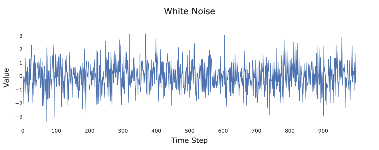
Figure 1:Simulated white noise process.
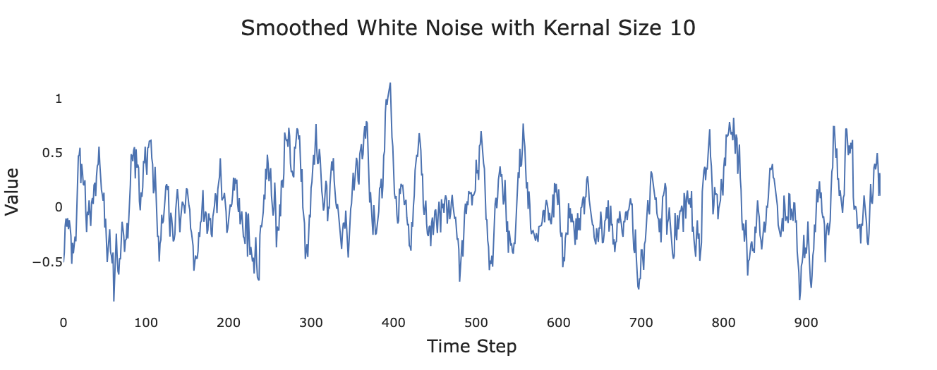
Figure 2:Smoothed version of white noise.
The following code lets you play around with different values for the noise and distributions. Note that if you are reading this in GitHub pages you will not be able to run the cell, you’ll either need to download the book or simpy copy and paste the code into a Jupyter notebook.
import numpy as np
import matplotlib.pyplot as plt

standard_deviation = 1.0 # Play around with this parameter!
white_noise = np.random.normal(loc=0.0, scale=standard_deviation, size=1000)
# We can also look at alternative distributions. Uncomment the following to use a Cauchy distribution instead.
# white_noise = np.random.standard_cauchy(size=1000)
plt.plot(np.arange(0, 1000, 1), white_noise)
plt.show()
Moving Average
Figure 1 and Figure 2 suggest one model for introducing temporal correlation in a series.
In a moving average (also known as a rolling average), each value is replaced by the average of that value and a selection of its neighbors.
Simple Three-Value Moving Average
For example, a simple centered three-value moving average would define as:
where is read as “is defined as.”
Even if the ’s are iid, the ’s will be serially correlated.
Example: Consider:
Both and depend on the values and , creating correlation between consecutive observations despite being iid.
Weighted Moving Average
Other weighting schemes are possible, for example:
This gives more weight to the central observation while still incorporating information from neighbors.
Random Walk
Applying a moving average to uncorrelated noise is one plausible method for introducing temporal correlation. Another scenario is when each time step starts from the value of the previous point (e.g., a stock price that opens trading at yesterday’s closing price).
Basic Random Walk
This suggests a model of the form:
where is the value of the series at time and the ’s are iid white noise.
Random Walk with Drift
If there is also an underlying trend (e.g., a stock’s long-term price going up), we can add a constant drift term :
Apparent Trends
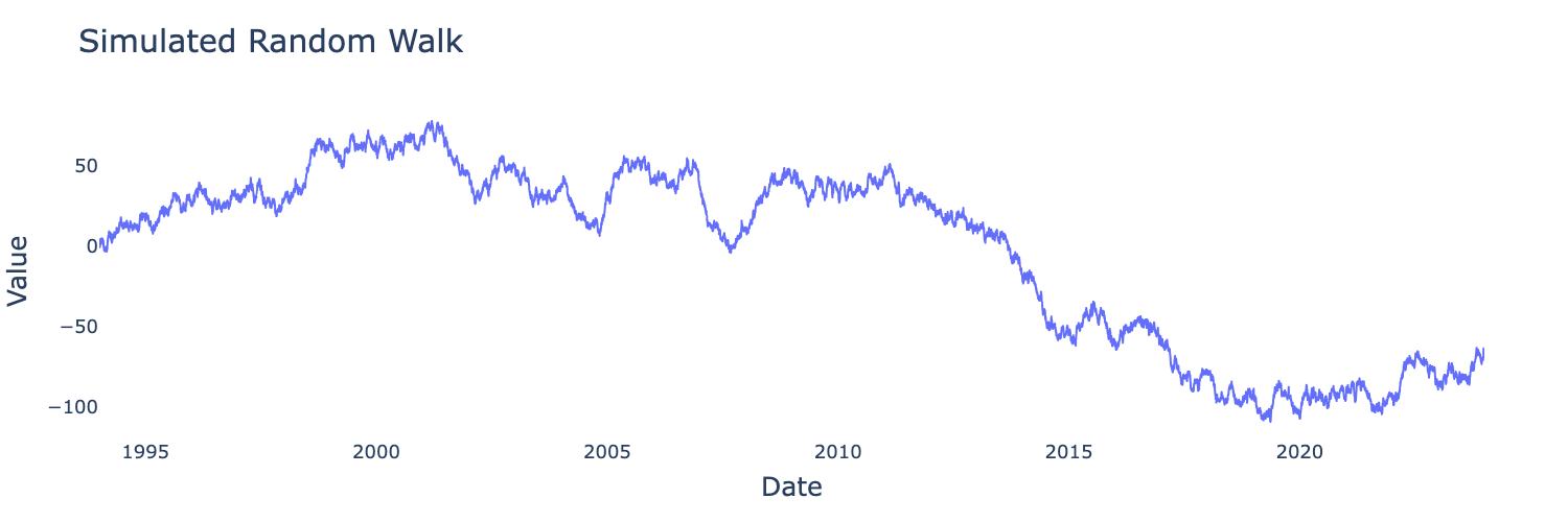
Figure 3:Simulated random walk with showing apparent trends.
We can simulate a random walk starting with our white noise and using the np.cumsum function—if you don’t understand why yet don’t worry, we’ll address it in later chapters. For now, this cell lets you get an idea of what random walks might look like. As before, you may need to copy and paste into a Jupyter notebook.
import numpy as np
import matplotlib.pyplot as plt

standard_deviation = 1.0 # Play around with this parameter!
white_noise = np.random.normal(loc=0.0, scale=standard_deviation, size=1000)
# We can also look at alternative distributions. Uncomment the following to use a Cauchy distribution instead.
# white_noise = np.random.standard_cauchy(size=1000)
plt.plot(np.arange(0, 1000, 1), np.cumsum(white_noise))
plt.show()
We will return to random walks and their cousins extensively throughout the book.
Autoregression
The concept of a random walk can be generalized to autoregressive processes.
Second Order Autoregression Example
Below we present a simulated autoregressive process generated by:
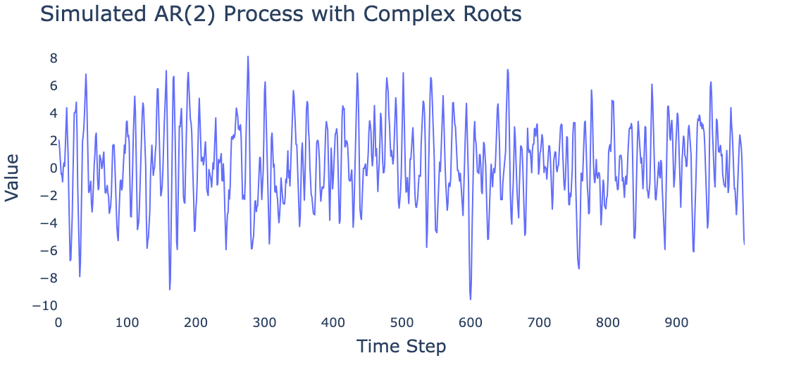
Figure 4:Simulated AR(2) process.
Note the long-range patterns, despite the fact that the model can only “remember” two time steps into the past. Autoregressive models have surprising ability to capture complex dynamics.
Signal and Noise
In many real-life scenarios, we consider our signal to be formed by the addition of white noise to an underlying process.
Separating signal from noise is a central focus in signal processing, with applications to:
Radar systems
Telecommunications
Sound engineering
Image processing
And many other fields
Example: Sinusoidal Signal with Noise
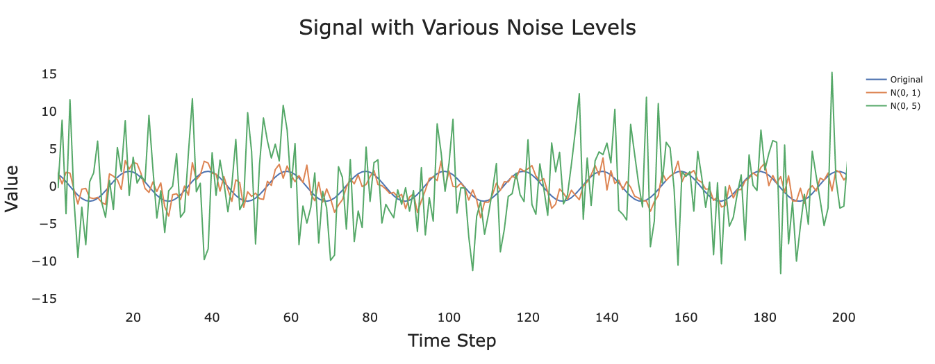
Figure 5:Signal for , , and .
As the variance of the noise increases, it becomes progressively more difficult to recover the underlying signal. Much of time series analysis is concerned with developing methods to extract meaningful patterns from noisy observations.