3.2 Autocovariance - Time Series Analysis for Data Scientists

Autocovariance Definition¶

As discussed in the first chapter, serial correlation of time series is both one the most challenging and most valuable aspects of time series. Autocovariance allows us to exploit serial correlation to address questions such as:

Is a high market close on one day indicative of a lower close the following day?
How long does a heat wave continue to skew temperatures above the norm?
Given higher sunspot activity this year, what year(s) in the future should we expect a repeat of this activity?

To give a concrete example, if we wish to know how strongly today’s highest temperature influences tomorrow’s, we may take the covariance of the series $(T_{0}, T_{1}, ...,T_{n-1})$ and $(T_{1}, T_{2}, ...,T_{n})$ , i.e.

\text{Cov}\Big(\sum_{i=0}^{n-1} T_i, \sum_{j=1}^{n} T_j \Big).

(1)

A high positive value for Eq. (1) tells us that higher (lower) temperatures today are indicative of higher (lower) temperatures tomorrow. While implausible for weather, in general many time series exhibit negative correlation, in which case a higher (lower) value at one time step is indicative of a lower (higher) value in the next.

We can naturally extent Eq. (1) to larger time lags to ask how long an anomalous temperature continues to skew the daily high. We will see in subsequent chapters that it is very common for time series to obey an exponentially decaying autocovariance.

Notation¶

Following the notation used in sources such as Shumway & Stoffer (2025) and Brockwell & Davis (2016), we will use the notation $\gamma_{x}(s, t)$ to denote the autocovariance at time lags $s$ and $t$ for time series $x$ :

\begin{split} \gamma_{x}(s, t) &\stackrel{\triangle}= \mathbb{E}[(x_{s}-\mu_{s})(x_{t}-\mu_{t})]\\ &=\mathbb{E}[x_{s}x_{t}]-\mu_{s}\mu_{t}\\ \end{split}

(2)

Note that $\gamma_x(s, t)=\gamma_x(t, s)$ .

In general, we will drop the $x$ subscript when it is obvious which time series we are referring to and only write $\gamma(s, t)$ . For an arbitrarily large (or infinite) observation window, $\mu_{s}=\mu_{t}$ as both series share almost all the same observations, leading to the simplification

\gamma(s,t)=\mathbb{E}[x_{s}x_{t}]-\mu^2\\

(3)

where we have dropped the subscript on $\mu$ .

Mean and Autocovariance of Moving Average¶

Recall from the first chapter that a white noise process is defined as a mean zero process with finite variance

w_t \sim wn(0, \sigma_w^2).

(4)

A summation of multiple values of $w_t$ will still have a mean of zero

\mathbb{E}[\ldots + w_{t-1}+ w_{t}+w_{t+1}+\ldots] = \dots+\mathbb{E}[w_{t-1}]+\mathbb{E}[w_{t}] + \mathbb{E}[w_{t+1}]+\ldots=0.

(5)

Consider the moving average

v_t = \frac{1}{3}(w_{t-1}+w_t+w_{t+1}).

(6)

$v_t$ has a mean of zero, but the autocovariance will depend on the difference between $s$ and $t$ :

\gamma_v(s, t)=\begin{cases} \frac{3}{9}\sigma_w^2, & s=t\\ \frac{2}{9}\sigma_w^2, & |s-t|=1\\ \frac{1}{9}\sigma_w^2, & |s-t|=2\\ 0, & \text{otherwise.}\\ \end{cases}

(7)

Note that even if all instances of the initial time series are iid, averaging will still introduce serial correlation.

Problem

Prove Eq. (7). Hint, since the $w_t$ ’s are iid, $\text{Cov}(w_i, w_j)=\delta_{ij}\sigma_w^2$ , where $\delta_{ij}$ is defined as 1 if $i=j$ and 0 otherwise.

Mean and Autocovariance of Random Walk¶

Mean for Zero Drift¶

Recall that a random walk (without drift) is defined as:

x_t = x_{t-1} + w_t

(11)

Iterating backwards, we have

\begin{split} x_t &= x_{t-1} + w_t\\ &= (x_{t-2} + w_{t-1}) + w_t\\ &= x_{t-2} + w_{t-1} + w_t\\ &= x_{t-3}+w_{t-2} + w_{t-1} + w_t\\ &\ldots\\ &=\sum_{h=0}^{\infty} w_{t-h} \end{split}

(12)

Of course, in real life we cannot have an infinite number of observations. Calling the first observation $w_0$ , this gives

\begin{split} x_t&=w_0+w_1+\ldots+w_t\\ &= \sum_{h=0}^{t} w_{t-h} \end{split}

(13)

Whether we use Eq. (12) or (13), the expectation value for the mean will always be 0, i.e.

\begin{split} \mathbb{E}[x_t] &= \mathbb{E}\Big[\sum w_{t-h}\Big]\\ &= \sum \mathbb{E}[w_{t-h}]\\ &=0. \end{split}

(14)

Mean with Drift¶

A random walk with drift is defined as

x_t = \delta + x_{t-1} + w_t, \qquad \delta \neq 0.

(15)

Following the same reasoning used above in Eq.s (12) and (13), we can iterate backwards to obtain

\begin{split} x_t &= \delta+x_{t-1} + w_t\\ &= \delta+(\delta+x_{t-2} + w_{t-1}) + w_t\\ &= 2\delta+x_{t-2} + w_{t-1} + w_t\\ &= 3\delta + x_{t-3}+w_{t-2} + w_{t-1} + w_t\\ &\ldots\\ &=t\delta + \sum_{h=0}^{t} w_{t-h} \end{split}

(16)

where we have only used the finite case to avoid $t\delta$ going to $\pm \infty$ .

The expectation value for Eq. (16) is

\begin{split} \mathbb{E}[x_t] &= \mathbb{E}\Big[t\delta+\sum_{h=0}^t w_{t-h}\Big]\\ &= \mathbb{E}[t\delta]+\sum_{h=0}^t \mathbb{E}[w_{t-h}]\\ &=t\delta. \end{split}

(17)

Random Walk Variance¶

Recall that while adding constants to random variables adjusts the means, it does not affect the variance or covariance, i.e.

\mathbb{V}(a+X) = \mathbb{V}(X),

(18)

and

\text{Cov}(a+X, b+Y) = \text{Cov}(X, Y),

(19)

thus the autocovariance of a random walk is independent of drift terms. To simplify notation we will therefore only explicitly address a random walk without drift.

Problem

Prove Eq.s (18) and (19).

The autocovariance at lags $s$ and $t$ is

\text{Cov}\Big(\sum_{i=0}^s w_i, \sum_{j=0}^t w_j\Big) = \text{Cov}(w_0, w_0) +\text{Cov}(w_0, w_1) +\ldots+\text{Cov}(w_s, w_t).

(22)

By the assumption of independent $w_t$ ’s, the only non-zero terms will be when $i=j$ (i.e. the variances). Assuming without loss of generality that $t\leq s$ , we have

\begin{split} \text{Cov}\Big(\sum_{i=0}^s w_i, \sum_{j=0}^t w_j\Big) &= \sum_{i=0}^t \mathbb{V}(w_i), \qquad t\leq s\\ &= t\sigma_w^2 \end{split}

(23)

From Eq. (23) we see that the variance of a random walk $\gamma(t,t)$ increases linearly with respect to $t$ , i.e.

\gamma(t,t) = t\sigma_w^2

(24)

equivalently, the standard deviation of a random walk increases with respect to $\sqrt{t}$

\text{s.d.} = \sqrt{t}\sigma_w

(25)

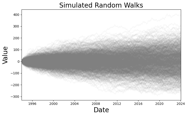
Figure 1 displays how random walks spread out with respect to time. Note how the random walks more closely follow a square root rather than a linear spread, which provides a concrete example of why standard deviation is often favored over variance in analysis.

1,000 simulated random walks with \sigma_w^2=1 and \delta=0. — Figure 1: $1,000$ simulated random walks with $\sigma_w^2=1$ and $\delta=0$ .

References¶

Shumway, R. H., & Stoffer, D. S. (2025). Time Series Analysis and Its Applications: With R Examples. In Springer Texts in Statistics. Springer Nature Switzerland. 10.1007/978-3-031-70584-7
Brockwell, P. J., & Davis, R. A. (2016). Introduction to Time Series and Forecasting. In Springer Texts in Statistics. Springer International Publishing. 10.1007/978-3-319-29854-2