Thus far, we have dealt with the theoretical values for various forms of variance, covariance, and correlation based on the assumption that we know the underlying process from which our observations have been drawn. In real life, we will usually be given the time series and then attempt to infer aspects such as the underlying process from statistical estimators. In this section we will develop techniques analogous to how sample covariance and sample correlation are used to estimate the true covariance and correlation in data science and statistics.
Estimate Definitions
Sample Autocovariance
The standard formula used in sources such as Shumway & Stoffer (2025) and Brockwell & Davis (1991) for sample autocovariance is
where is the sample mean and the “hat” notation indicates that is an estimate of the true population value. Note that we assume the same mean for and .
Sample Autocorrelation
Autocorrelation is estimated by defining the sample autocorrelation
Sample Cross-Covariance
The sample cross-covariance is defined as
and the sample cross-correlation as
Properties of Estimators
Positive Semidefiniteness
You may have noticed something strange about Eq. (1). For observations, we only have pairs to sum over; for example when and there are 98 pairs consisting of . Why then, do we divide Eq. (1) by rather than ?[1]
The answer relates to the necessity that the autocovariance matrix (and by extension autocorrelation matrix) be positive semidefinite in order to avoid the possibility of generating negative variances. To see that the form used in Eq. (1) guarantees this property, let us sketch the proof from Brockwell & Davis (2016)[2]. Let us define the matrix using the demeaned time series such that
where the elements of are the vectors appropriately padded with zeros. Put slightly differently, we have now factored such that
Since we have expressed as the square of , for any vector we have
The central point to understand is that we could only factor because we could pull out from every entry. If we separately weighted each in by , we would no longer be able to express the autocovariance matrix as the product of two other matrices. Consequently, we would have no guarantee that was positive semidefinite, and could end up with negative variances.
Bias and Consistency
Note that neither dividing by nor creates an unbiased estimator, i.e. in neither case is it true that
though when dividing by the bias will be smaller.
The estimates are both, however, consistent in that in as
As observed in Wasserman (2004), most modern statistics texts consider consistency to be sufficient and are less concerned with estimators being unbiased.
Standard Error of Autocorrelation and Cross-Correlation
A natural question to ask is how we might determine if an autocorrelation value is statistically significant. We previously touched on the fact that programs such as statsmodels estimate statistical significance automatically. But we have not yet explained how significance is estimated.
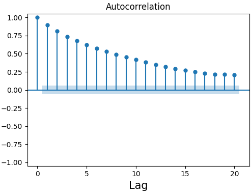
Figure 2:Sample autocorrelation plot from statsmodels with blue shading indicating area of statistical insignificance.
It turns out that in order to definitively calculate statistical significance, we would need to know the underlying process that generated our data—exactly the question we are trying to answer in the first place. Instead, let’s ask a slightly different question: What values should we expect for the autocorrelation if our time series is pure white noise?
Under the assumption of white noise[3], we can expect the sample autocorrelation values to be normally distributed with mean 0 and variance
where is the total number of observations (Box et al. (2008)). Equivalently, the standard error of is given by
For a white noise process, we expect around of all sample autocorrelation values to fall within . By default, statsmodels usually uses Eq. (13) at a confidence interval to estimate statistical significance to create figures such as Figure 2[4]. It can be shown that this formula also holds for estimating the sample cross-correlation (Shumway & Stoffer (2025)).
While Eq. (1) is the default method for calculating sample autocovariance in
statsmodels, the autocovariance and autocorrelation (found instatsmodels.tsa.stattools.acovfandstatsmodels.tsa.stattools.acf, respectively) have an argumentadjustedthat can be set toTruein order to divide by instead. By default, both functions setadjusted=False(i.e. dividing by by default). The cross-covariance and cross-correlation functions instatsmodelsdefault toadjusted=Trueas they do not share the same requirement to be positive semidefinite. Our definition in Eq. (6) follows sources such as Box et al. (2008) and Shumway & Stoffer (2025).The full proof is unnecessary for our purposes, but can be found in Sec. 2.4.2 of the referenced text for those who are interested.
Strictly, this formula is only valid for noise with a finite fourth moment such as Gaussian white noise (Shumway & Stoffer (2025)). As the formula is in any event an approximation for any non-white noise time series we will not be too concerned about this point.
statsmodelscan be forced to always use this method by settingbartlett_confint=False.
- Shumway, R. H., & Stoffer, D. S. (2025). Time Series Analysis and Its Applications. In Springer Texts in Statistics. Springer Nature Switzerland. 10.1007/978-3-031-70584-7
- Brockwell, P. J., & Davis, R. A. (1991). Time Series: Theory and Methods. In Springer Series in Statistics. Springer New York. 10.1007/978-1-4419-0320-4
- Brockwell, P. J., & Davis, R. A. (2016). Introduction to Time Series and Forecasting. In Springer Texts in Statistics. Springer International Publishing. 10.1007/978-3-319-29854-2
- Wasserman, L. (2004). All of Statistics: A Concise Course in Statistical Inference. In Springer Texts in Statistics. Springer New York. 10.1007/978-0-387-21736-9
- Box, G. E. P., Jenkins, G. M., & Reinsel, G. C. (2008). Time Series Analysis. In Wiley Series in Probability and Statistics. Wiley. 10.1002/9781118619193
- Box, G. E. P., Jenkins, G. M., & Reinsel, G. C. (2008). Time Series Analysis. In Wiley Series in Probability and Statistics. Wiley. 10.1002/9781118619193