As discussed in Chapter 2, covariance, and by extension autocovariance, has some undesirable characteristics. For this reason, in time series analysis we often prefer to work with the autocorrelation, which is a unitless quantity bounded by [−1,1].
For any finite variance process, the autocorrelation is simply the autocovariance normalized by the the variances.
γ(0) is the variance, and hence cannot be negative, so vTPv will only differ from vTΓv by a positive constant term given by γ(0)1. As a result, since Γis positive semidefinite, P must also be as well.
It is often instructive to plot the autocorrelation of a time series. statsmodels has a nice built-in function to create plots:
from statsmodels.graphics.tsaplots import plot_acf
plot_acf(my_time_series, lags=20)
where the parameter lags controls the maximum value of h. lags=20 is generally a good starting choice for most scenarios, though for longer patterns such as hourly data with a 24-hour period you may want to set lags to something like 72 or 96.
plot_acf has other arguments that we will discuss once we’ve covered more theory. For now, let’s take a look at a couple of different autocorrelation plots to get a feeling for how they behave.
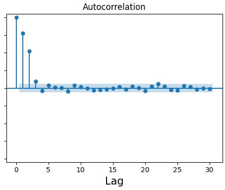
Figure 1:Sample autocorrelation plot from statsmodels with sudden cutoff point. Note that lag 0 is always equal to 1.
Figure 1 shows two significant lags (plus the value of 1 at h=0), and falls to statistical insignificance thereafter as denoted by the blue shading. Later on we will see that this is a hallmark characteristic of a moving average process.
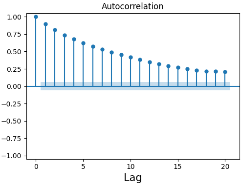
Figure 2:Sample autocorrelation plot from statsmodels with exponential decay.
Figure 2 demonstrates an exponentially decaying autocorrelation that remains statistically significant even at h=20. In later chapters we will see that this behavior corresponds to an autoregressive process.