Kernel Smoothing
We’ve encountered data smoothing in the form of a moving average. Figure 1 and Figure 2 present a synthetic white noise process and the same process after smoothing with a moving average of length 10.
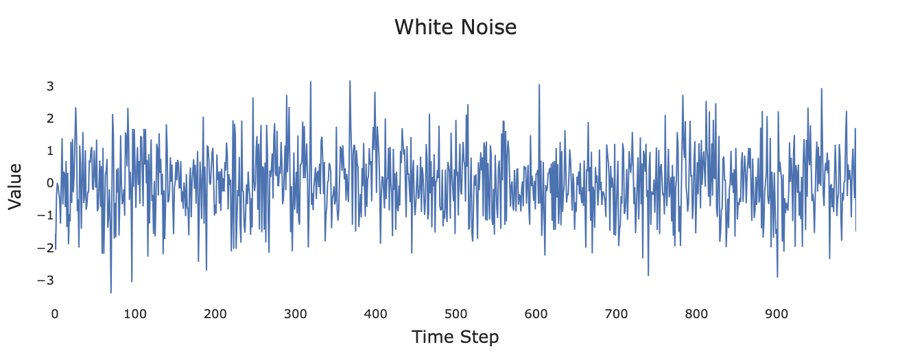
Figure 1:Simulated white noise process.
![Smoothed version of white noise after applying the filter [\frac{1}{10}, \frac{1}{10},...,\frac{1}{10}].](/time-series-book/build/smoothed_white_noise-9ebda525cd9be2443518a02f96308935.png)
Figure 2:Smoothed version of white noise after applying the filter .
We can think of the smoothing process depicted in Figure 2 as consisting of sliding a kernel (also known as a filter) across the data. In this case, the kernel is defined as
which we can envision as being slid across the data. At each point, we take the inner (or dot) product of the data with the kernel. For the kernel used in Eq. (1) this gives the unweighted average of 10 points. In later chapters we will learn that this can be thought of as a convolution in the frequency domain.
The box (or boxcar) kernel used in Figure 2 is only one of many possible choices. We will learn in future chapters that a box filter has substantial shortcomings in the frequency domain that are mitigated (though not eliminated) by use of tapered kernels, such as kernels based on Gaussians, the cosine function, or the tricube function introduced in the next section.
Tricube Function
For this chapter, the most important kernel method is generated from the tricube function :
where is the distance between the the focal point and the point calculated as [1]. The maximum is determined by an adjustable parameter giving the length of the kernel.
For example, for , the tricube function generates a sharply peaked kernel with non-zero values out of total values
with all points outside the window weighted as 0 (note that for the first and last elements , resulting in zero for ). In actual implementation we would simply use a kernel of length (9, in our example) instead of using a kernel of length (11, in our example) with zeros in the first and last positions. We explicitly included the zeros in Eq. (3) to emphasize that the kernel falls to zero at .
Weighting Points Near the Edges
In order to avoid shortening the time series (as occurs with moving averages), any point less than from either end has an asymmetric selection of points in order to maintain the same kernel size at the expense of a larger value for . For example, continuing with from before, the asymmetric window used for the first point in the series will now have with values given as:
LOWESS Algorithm
Local regression is perhaps best thought of as a hybrid between kernel smoothing and linear regression (or more broadly polynomial regression). The most common family of methods is LOWESS (locally weighted scatterplot smoothing), a type of LOESS (locally estimated scatterplot smoothing)[2]. The LOWESS algorithm is generally credited as having been formally introduced in Cleveland (1979) and Cleveland (1981) (though much of the concept had been proposed independently by Savitzky & Golay (1964) about fifteen years beforehand).
LOWESS Demo
Before diving into the underlying algorithm, let’s get a feeling for how LOWESS behaves. The following interactive figure plots the function
for some noise in gray dots. For reference, the original (presumably unknown) clean signal without noise that we are attempting to reconstruct is denoted by a gray dashed line. The toggle button LOWESS CURVE turns on or off the LOWESS curve fitted through the points. The button LOCAL FITS toggles on and off a selection of the individual local regression lines (more on those soon). Finally, the slider SPAN (f) tells the algorithm what fraction of the overall data to consider for each local fit. Note that at 1.00, the line is almost a flat linear regression line with large local regression lines. As you shrink the fraction down, the LOWESS fit becomes more jagged with smaller local regression lines (denoting that the local line is calculated with a smaller portion of the data).
If the above fails to render correctly in your browser you can also open the demo as a new browser window using the Open Demo in a New Tab ↗ button at the top of the frame. Note that you may need to enable popups for this to work.
Local Regression
The LOWESS algorithm begins by dividing the data into overlapping windows. The size of each window is governed by the parameter , the fraction of the total observations . In statsmodels.nonparametric.smoothers_lowess.lowess, the fraction is set with the argument frac (default frac=2.0/3.0). In the demo above, can be smoothly varied from 0.05 to 1. Once is chosen, we create windows of length centered at each data point where is the ceiling function indicating the smallest integer greater than or equal to . For each window about a given central point (denoted as ), we calculate a weighted linear regression defined as
where is a weight function, most commonly the tricube function, that weights the contribution of each based on its distance from and where we have expressed the coefficients as and to emphasize that distinct ’s are calculated for each data point. For points closer than to either end, the window no longer places the point in the center of the window, and uses the modification to discussed above.
LOWESS can be extended from linear regression to polynomial regression using expressions such as
though we will not need to go beyond Eq. (6) for our purposes.
Having calculated distinct linear regressions, we use each linear regression about a given to calculate the at that point, leaving us with values (one per data point). The points are then connected into a single curve—though note in the demo above that the fitted curve becomes notably more jagged as is decreased.
Robust Smoothing
In the demo above, we calculated the LOWESS curve solely by implementing Eq. (6). This method works well for data that has relatively few outliers. Cleveland (1979) describes an optional second stage of smoothing using the bisquare function defined as
where as in Eq. (2) falls to zero at . After the initial LOWESS curve calculation using Eq. (6), the algorithm then goes through a predetermined number of iterations of the following procedure:
Calculate the residual between the predicted and observed points
Determine new weightings for each point by first calculating the median of the 's and then applying the formula
Recalculate the local regressions using Eq. (6) using instead of .
Cleveland refers to this algorithm as “robust locally weighted regression.” In statsmodels, the number of iterations of the above procedure is controlled by the argument it (default it=3). Setting it=0 will result in the algorithm
only using Eq. (6) in its original form.
In general, robust smoothing is primarily required for datasets with large outliers, such as those produced by Cauchy distributed noise. Figure 3 demonstrates LOWESS smoothing with different numbers of iterations on a synthetic dataset with Cauchy distributed noise. Note in particular that for 0 iterations (non-robust LOWESS) the fitted LOWESS line “chases” the outliers out of the plot. Once we reach 3 iterations, the LOWESS line almost perfectly captures the original signal.
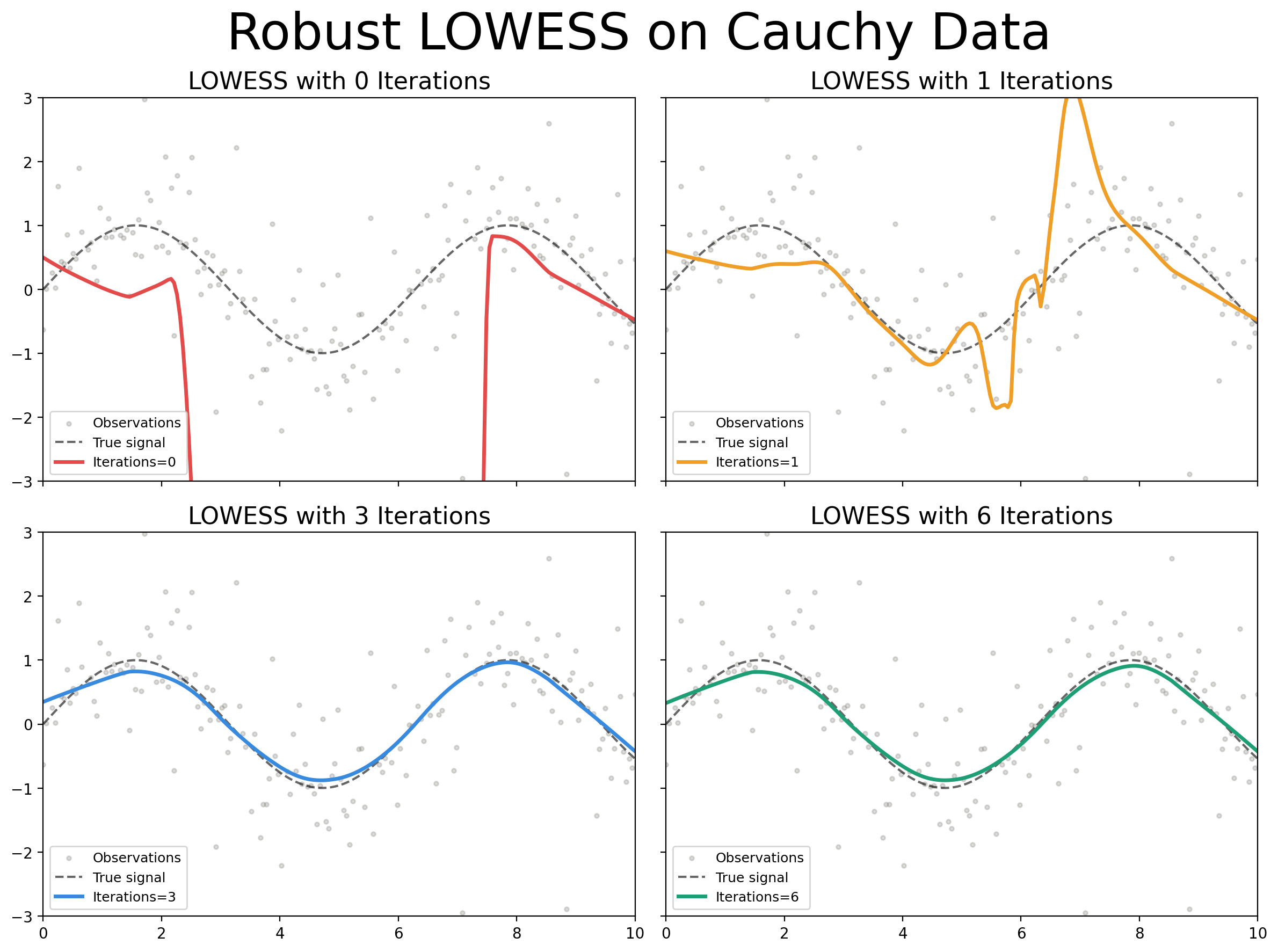
Figure 3:LOWESS regression using and 6 iterations of robust smoothing on synthetic dataset defined as with Cauchy distributed.
The quantity is often referred to as the bandwidth. We will reserve the term bandwidth for use in the context of the frequency domain.
Some sources such as NIST treat the terms LOESS and LOWESS as being interchangeable. Cleveland himself in Cleveland & Devlin (1988) appears to have used the term LOESS as a multivariate generalization of the previous univariate LOWESS.
- Cleveland, W. S. (1979). Robust Locally Weighted Regression and Smoothing Scatterplots. Journal of the American Statistical Association, 74(368), 829–836. 10.1080/01621459.1979.10481038
- Cleveland, W. S. (1981). LOWESS: A Program for Smoothing Scatterplots by Robust Locally Weighted Regression. The American Statistician, 35(1), 54. 10.2307/2683591
- Savitzky, Abraham., & Golay, M. J. E. (1964). Smoothing and Differentiation of Data by Simplified Least Squares Procedures. Analytical Chemistry, 36(8), 1627–1639. 10.1021/ac60214a047
- Cleveland, W. S., & Devlin, S. J. (1988). Locally Weighted Regression: An Approach to Regression Analysis by Local Fitting. Journal of the American Statistical Association, 83(403), 596–610. 10.1080/01621459.1988.10478639