Having explained classical approaches to time series decomposition and local regression, we are now in a position to understand how Seasonal-Trend decomposition using LOESS[1] (STL). Cleveland et al. (1990) from Bell Labs and the University of Michigan introduced STL to compensate for the shortcomings of classical decomposition. As we shall see, STL grows naturally out of augmenting classical decomposition with LOESS. Using LOESS gives the flexibility to calculate trends for all data points, unlike moving averages which truncate the first and final values. Furthermore, unlike the X-11 family which only handles quarterly or monthly seasonalities, STL can handle any number of seasons per cycle.
STL Algorithm
Log Transformation
Unlike with classical decomposition, STL only works with additive trend and seasonal components. Data with a multiplicative trend must be log transformed to use STL. In practice, this is rarely a major impediment to using STL, though applying a log transform does cause interpretability to go slightly down.
STL Loops
The STL algorithm runs a nested loop of functions until the algorithm reaches a set stopping point determined by the user’s choice of both inner and outer loops. We will defer discussion of deseasonalization for the moment to first understand the overall procedure. Letting be the number of passes in the inner loop and be the number in the outer loop, the algorithm is as follows:
Initialize robustness weights for LOESS to 1 and the trend to 0.
1.1 Detrend the series using the most recently calculated trend (set at 0 initially).
1.2 Divide the data into subseries (e.g. the first subseries consisting of each January, the second subseries consisting of each February, etc.). Generate LOESS (weighted by robustness) curves independently for each subseries to smooth the detrended data.
1.3 Calculate the seasonal component (next section) and deseasonalize the data.
1.4 Apply another round of (weighted) LOESS on the deseasonalized data to determine the trend to be used as the starting point for the next iteration.
1.5 Return to step 1.1 until completing passes.
Calculate the residuals. If , calculate robustness weights to quantify each residual’s degree of extremity for the LOESS algorithm (i.e. to what extent it should be considered an outlier) and return to step 1.1 until completing iterations, otherwise stop.
The fact that LOESS can output smoothed data with the same length as the original data is crucial for steps 1.2 and 1.4. With a standard moving average, each pass of a length filter would delete ( even) or ( odd) observations; running multiple loops on a small dataset would quickly whittle it down to nothing. It is only because we use LOESS that we can freely run the inner loop for multiple iterations. Additionally, note that the use of distinct subseries in step 1.2 allows the magnitude of each seasonal component to vary over time.
By default, statsmodels does not use robust fitting (i.e. ) and uses 5 inner loops (). This can be changed by setting robust=True, which by default will use and . and can also be set manually in the fit method by calling STL(data).fit(inner_iter=n_i, outer_iter=n_o).
STL Deseasonalization
In step 1.3 we referenced deseasonalization without explaining how this is performed. A major advantage of STL over classical decomposition is that it allows the magnitudes of the seasonal component to vary over time instead of locking us into a single set of seasonal magnitudes for the entire series. The algorithm used in 1.3 functions as follows:
The deseasonalization step starts by creating an intermediate series consisting of the results of step 1.2 reassembled from the constituent subseries and temporarily padded at both ends.
is calculated from by smoothing with a three step “low-pass” filter[2] consisting of two sequential unweighted moving averages of length , followed by an unweighted moving average of length 3 (which together remove the padding from step 1), and finishing with LOESS.
Seasonal components are calculated as (using the non-padded ). Subtracting removes low-frequency long-term components from the seasonality, leaving solely the short-term seasonal effects in . is then subtracted from the series for this iteration’s deseasonalized series.
An important advantage of STL is that, while we do still need to specify an value for the seasonal length, we are no longer constrained to have a single average per season as we were in classical decomposition. Instead, the use of LOESS in step 2 allows for variations in the magnitudes of the seasonal component (though not its length) over the course of the data.
Plotting STL Decomposition Components
Plotting the default statsmodels implementation of STL results in Figure 1:
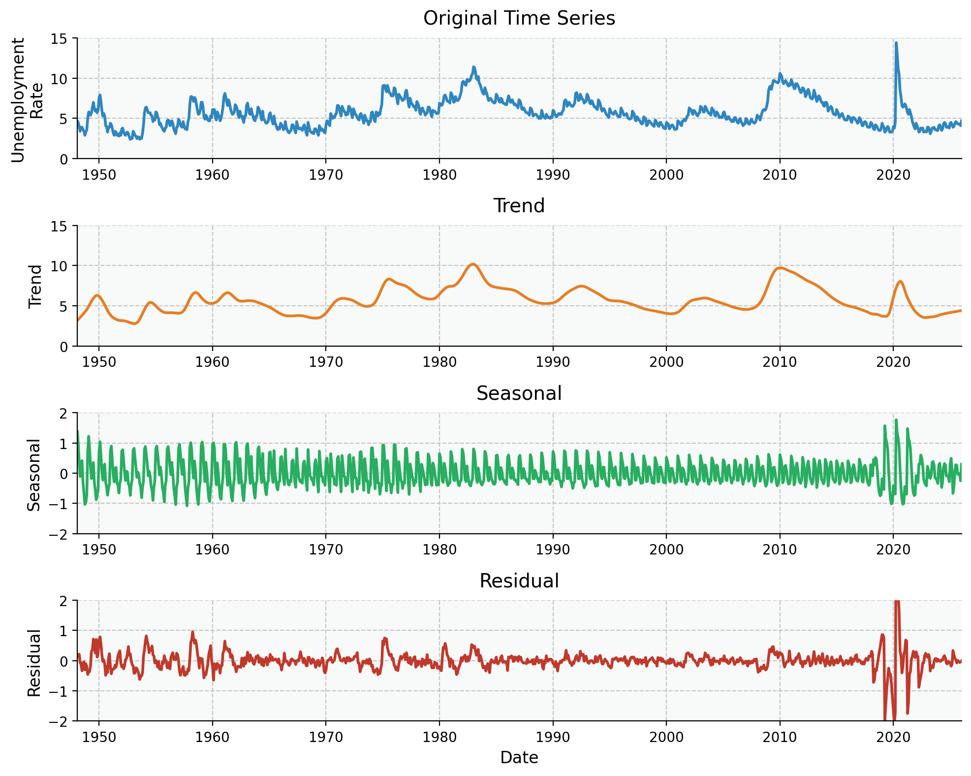
Figure 1:US employment rate from 1948 through 2025 from the Federal Reserve Bank of St. Louis with STL decomposition using the default settings in statsmodels of and . Plot consists of original series (top), trends and cycles (second from top), seasonal contribution (third from top), and residual variation not explained (bottom).
Applying the assessment method from classical decomposition results in and . Compared with the classical decomposition results of and , this indicates that STL has done a marginally better job isolating the trend but a substantially better job isolating the season component.
Multiple Time Scales
As presented, STL can only decompose a single seasonality. Bandara et al. (2021) generalize STL to handle multiple seasonal lengths (e.g. both a daily and yearly seasonality in temperature) in Multiple Seasonal-Trend decomposition using LOESS (MSTL). MSTL was implemented in statsmodels as statsmodels.tsa.seasonal.MSTL in version 0.14.0 released in May of 2023. While MSTL can be a useful tool, in practice it is not currently widely adopted. In general, I would usually recommend use of frequency domain techniques for analyzing multiple seasonal lengths in a single time series. While not as immediately interpretable as STL or MSTL, frequency domain methods more than make up for the increased complexity with their tremendous ability to tease out the contributions of different seasonal trends.
Cleveland et al. (1990) write that the “L” stands for LOESS. We will maintain this terminology, though for the purposes this book we will only need the narrower univariate LOWESS algorithm rather than the multivariate LOESS.
We will explore why this filter is referred to as “low-pass” in the chapter covering the frequency domain.
- Cleveland, R. B., Cleveland, W. S., McRae, J. E., & Terpenning, I. (1990). STL: A Seasonal-Trend Decomposition Procedure Based on Loess. Journal of Official Statistics, 6(1), 3–73.
- Bandara, K., Hyndman, R. J., & Bergmeir, C. (2021). MSTL: A Seasonal-Trend Decomposition Algorithm for Time Series with Multiple Seasonal Patterns. arXiv. 10.48550/ARXIV.2107.13462