4.5 Increasing Variance and the Log Transform - Time Series Analysis for Data Scientists

Most of the time series we’ve seen so far have had constant variance across time^[1]. In some scenarios, particularly those involving exponential growth, variance may increase concomitantly with the value. For example, as overall air travel increases, the absolute difference between busier and less busy seasons will also increase (even if the relative difference is constant). Such time series are non-stationary for at least two (and often three) reasons:

The mean is non-constant over time.
The variance $\gamma(0)$ is non-constant over time.
Some examples such as air travel may also be non-stationary due to seasonal effects.

Apple Mac Sales¶

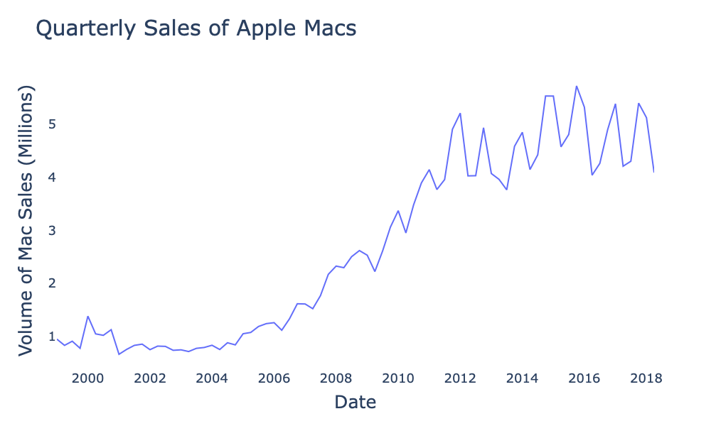
Figure 1:Quarterly sales figures for Apple Mac computers in millions from GitHub Apple Data Repository.

Figure 1 appears to be non-stationary for all three reasons listed above. The mean shows a steady upward trend and the volumes appear to exhibit a seasonal effect with higher sales in the autumn and winter and lower sales in the spring and summer. As the size of the seasonal effect appears to depend on the overall trend, the variance also increases with time.

Let’s first address the increasing variance by replacing the raw values with their logarithms:

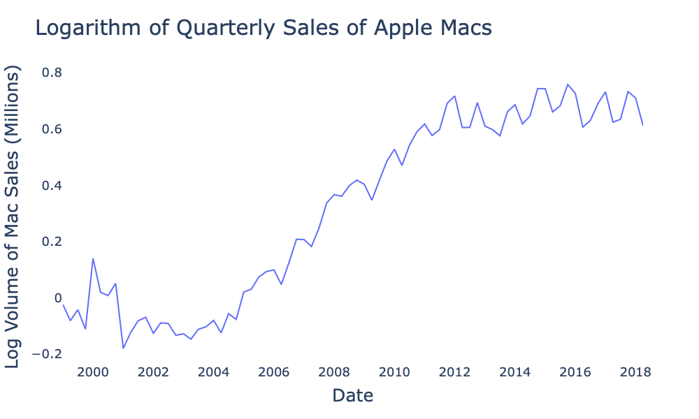
Figure 2:Logarithm of quarterly sales figures for Apple Mac computers in millions from GitHub Apple Data Repository.

Figure 2 is beginning to look better—the variance appears to be roughly constant across time. We can address both the trend and seasonality by taking the first and fourth differences of the log values, i.e.

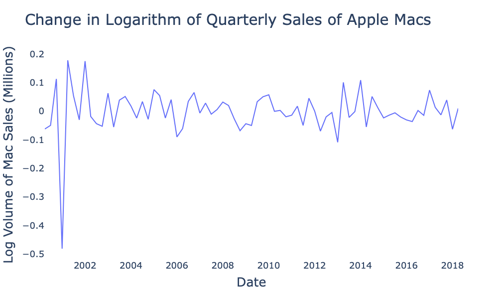
z_t \overset{\triangle}{=} \nabla_4\,\nabla\big(\log{(x_t)}\big)

(1)

Figure 3:First and fourth differences of logarithm of quarterly sales figures for Apple Mac computers in millions from GitHub Apple Data Repository.

Figure 3 certainly looks stationary upon visual inspection. After we’ve covered autoregressive processes we will revisit this example with statistical tests designed to help determine stationarity.

Problem

In Eq. (1) we applied the first difference at lag 1 followed by the first difference at lag 4. Would it have made a difference if we’d switched the order and instead used $\nabla\,\nabla_4\big(\log{(x_t)}\big)$ ?

Log Difference and Returns¶

In Eq. (1) we used the first (and fourth) difference of the logarithm of the sales figures. This concept closely relates to the return, a unitless quantity defined as the difference in value between successive time steps divided by the previous time step, i.e.

r_t \overset{\triangle}{=} \frac{x_t-x_{t-1}}{x_{t-1}}.

(5)

To see this relation, let us rewrite Eq. (5) as

\frac{x_t}{x_{t-1}} = 1+r_t.

(6)

We now have

\begin{split} \nabla \log{(x_t)} &= \log{(x_t)}-\log{(x_{t-1})}\\ &= \log{\Big(\frac{x_t}{x_{t-1}}\Big)}\\ &= \log(1+r_t)\\ &\approx r_t \end{split}

(7)

where we have used the Taylor expansion

\log{(1+r_t)} = r_t -\frac{r_t^2}{2}+\dots

(8)

Under the assumption of small $r_t$ , quadratic and higher order terms will be negligible. Figure 4 demonstrates that the two functions are essentially identical for returns with an absolute value less than about $20\%$ . For this reason, $\nabla\log{(x_t)}$ is often used interchangeably with the return defined in Eq. (5).

Linear slope y=r_t (gray) and logarithmic curve y=\log{(1+r_t)} (blue) for r_t\in[-0.5, 0.5]. — Figure 4:Linear slope $y=r_t$ (gray) and logarithmic curve $y=\log{(1+r_t)}$ (blue) for $r_t\in[-0.5, 0.5]$ .

Footnotes¶

A random walk is an important exception. Random walks have a linearly increasing variance with respect to time.
↩