4.4 Time Series with Seasonality - Time Series Analysis for Data Scientists

Seasonality Definition¶

One of the defining characteristics of time series is the presence of seasonality. Put simply, seasonality is a regular and predictable variation in a time series. Some examples of seasonal effects are:

Higher temperatures during the day than the night
Higher temperatures in July than January (in the northern hemisphere)
Unemployment rates increasing in January after the holiday season
Higher traffic density on weekdays than weekends

Note that multiple seasonal effects of different time scales may be layered together, for example higher temperatures during the day combining with higher temperatures during the summer.

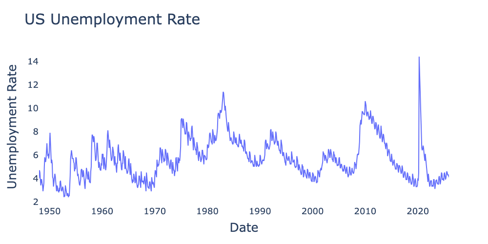
Figure 1:US employment rate from 1948 through 2025 from the Federal Reserve Bank of St. Louis (not seasonally adjusted).

A time series with seasonal effects is not stationary because its mean is dependent on time. For example, Figure 1 is not stationary because the expectation value for unemployment is consistently higher in January.

Seasonal vs. Cyclic Changes¶

It is important to distinguish between seasonal effects and cyclic effects. They both describe periodic fluctuations in a time series, but are distinguished by regularity.

Seasonal and cyclic effects are also sometimes distinguished by cycle length, in particular in econometrics. Behavior with a period of up to a year is often binned as seasonal, whereas behavior with periods longer than a year or two is binned as cyclic. It is important to understand that this is a common characteristic, not a definition. Nothing inherently precludes the existence of seasonal effects with periods far longer than a year or cyclic effects with periods far shorter than a year.

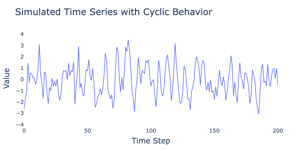
Figure 2:Simulated time series showing strong cyclical behavior with irregular repetition frequency.

Figure 2 shows a simulated time series with strong periodic behavior. However, since the periodicity is not constant, the underlying process is still stationary. In future chapters we will learn that this is a hallmark of autoregressive (AR) processes with complex roots.

Distinguishing Seasonal and Cyclic Effects¶

So how do we know if a periodic effect is seasonal (and hence makes the time series non-stationary) or cyclic (and does not affect stationarity)? Some cycles such as Figure 2 or the multi-year cycles in Figure 1 are fairly easy to identify as not being seasonal. On the other hand, how do we verify that effects such as the yearly cycles in unemployment are seasonal and not cyclic? While there is no foolproof way to demonstrate that an effect is seasonal, there are a few tools we can use to help:

High regularity: When we have a long time series such as Figure 1 that covers over 75 years, the extreme regularity of January spikes is almost certainly a seasonal effect. However, if we only had 10 years of so to examine and/or had a much noisier time series, regularity would not be as strong an indicator.
Domain expertise: As with much of data science, we seek to incorporate priors from domain expertise. For example, it is quite reasonable to assume annual effects leading to an increase in unemployment in the same month every year. In contrast, had we seen an effect with, say, a seven month period, it would be less likely to have been a true seasonal effect.
Autocorrelation: The autocorrelation function for cyclic effects tends to display an exponential decay with sinusoidal behavior, such the autocorrelation function for Figure 2 shown in Figure 3:
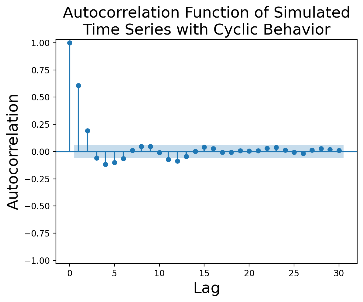
Figure 3:Autocorrelation function for simulated cyclic time series.
In contrast, the autocorrelation function for the first difference^[1] of Figure 1 shows marked spikes with a twelve-month periodicity:
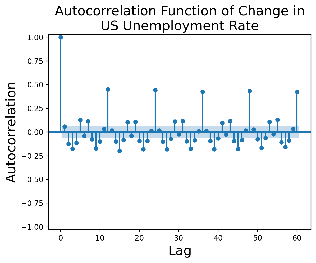
Figure 4:Autocorrelation function of change in US employment rate from 1948 through 2025 from the Federal Reserve Bank of St. Louis (not seasonally adjusted).
Be aware that for most time series you’re likely to encounter in real life, the autocorrelation function is likely to be far more ambiguous than the examples above.

Problem

In this problem you will examine an example of an autocorrelation function that may not be as easy to categorize as reflecting either seasonal or cyclic behavior. statsmodels has a preloaded time series dataset of historical sunspot activity, load it into a dataframe and plot the autocorrelation using the following code:

import statsmodels.api as sm
from statsmodels.graphics.tsaplots import plot_acf

sunspots_df = sm.datasets.sunspots.load_pandas().data
sunspots_df.index = pd.Index(pd.date_range("1700", end="2009", freq="YE-DEC"))
sunspots_df.drop(columns="YEAR", inplace=True)
plot_acf(sunspots_df, lags=50)

Does the plot of the autocorrelation function resemble either Figure 3 or Figure 4? What conclusions would you draw regarding the periodicity of sunspots?

In subsequent chapters, we cover additional methods for identifying seasonality using time series decomposition and Fourier analysis.

Methods for Addressing Seasonality¶

There are two major reasons we might want to remove seasonal effects from our time series:

Seasonal effects result in non-stationary time series, whereas methods such as the ARMA family require stationarity.
We may wish to identify long-term patterns and trends that can be obscured by normal seasonal fluctuations.

We will cover three major methods of removing seasonal effects.

Seasonal Moving Average¶

The first approach is arguably also the most intuitive, namely taking a moving average (also known as a rolling average) of our time series values with a window equal to the length of the “season.” For example, if we are focused on daily temperatures but have hourly data, we might take a 24-hour moving average such that the first hourly value in our series is the mean of hours $0-23$ , the second value is the mean of hours $1-24$ , and so on.

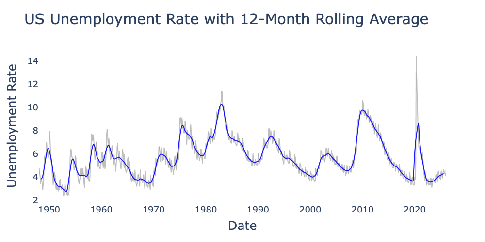
Figure 5:US employment rate from 1948 through 2025 from the Federal Reserve Bank of St. Louis with raw data (gray) and a centered 12-month moving average (blue).

Seasonal Adjustment¶

Seasonal adjustment is a central technique in econometrics and is used heavily by organizations such as the Federal Reserve Bank. We will defer a complete discussion of seasonal adjustment until next chapter; for now we may think of it as defining a set seasonal effect $S_t$ for each season and adjusting the time series to remove it. Seasonal adjustment is performed via one of two major methods:

Additive: By far the more common method, additive models assume our time series can be adjusted by subtracting $S_t$ :
$y_t = x_t - S_t,$
(1)
where for example we might calculate that January is 20 degrees colder than average and July is 25 degrees hotter, giving
$\begin{align*} S_{January} &= -20\\ &\ldots\\ S_{July} &= 25\\ &\ldots \end{align*}$
(2)
Multiplicitive: Less commonly, we might instead assume our time series can be seasonally adjusted by dividing by $S_t$ :
$y_t = \frac{x_t}{S_t}.$
(3)
Multiplicative seasonal adjustment most commonly applies in scenarios showing exponential growth such as stock or commodity prices (without adjustment for inflation). Relative prices for gasoline might consistently be a few percentage points higher in the summer than the winter, but the absolute price difference in 2026 is likely to be substantially greater than the absolute difference in 1976.

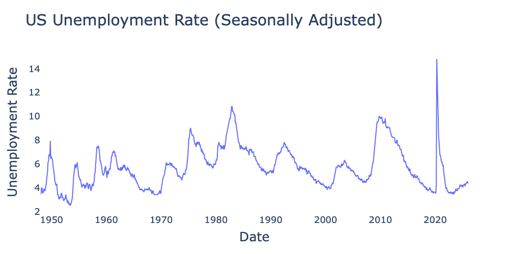
Figure 6:US employment rate from 1948 through 2025 from the Federal Reserve Bank of St. Louis using Federal Reserve Bank’s seasonal adjustment method.

Seasonal Differencing¶

The final method we will use is seasonal differencing. We have seen how the first difference removes random walk characteristics. By the same token, we may build a model consisting of a seasonal random walk in which the current season’s value is determined by last season’s value plus some noise $w_t$ . For example, we might propose a monthly model

\begin{align*} x_{January,\, t} &= x_{January,\, t-1} +w_{January,\, t}\\ x_{February,\, t} &= x_{February,\, t-1} +w_{February,\, t}\\ &\vdots \end{align*}

(6)

where $t$ refers to the current year and $t-1$ to the previous year. Allowing that Eq. (6) is a valid representation of the underlying process generating our time series, the natural method to compensate for its effects is to take the seasonal difference $\nabla_s$

\begin{split} z_t &\overset{\triangle}{=} \nabla_s\,x_t\\ &= x_{t}-x_{t-s}\\ &= (1-\mathbb{B}^{s})\,x_t \end{split}

(7)

where $s$ is the number of seasons per period; in the case of monthly data we have $s=12$ giving us $\nabla_{12}$ .

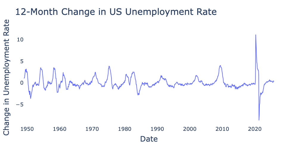
Figure 7:US employment rate from 1948 through 2025 from the Federal Reserve Bank of St. Louis after applying 12-month differencing.

Figure 7 shows the 12-month change in the US unemployment rate. While it still demonstrates cycles varying from around five to ten years in duration, these do not negate stationarity. Figure 8 shows the autocorrelation function for the series in Figure 7. The sinusoidally decaying nature of the autocorrelation is consistent with a stationary cyclic time series.

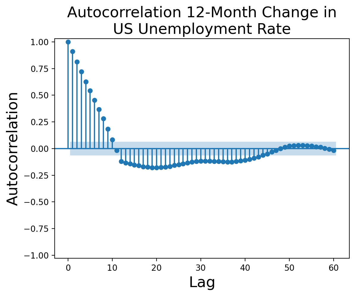
Figure 8:Autocorrelation function of US employment rate from 1948 through 2025 from the Federal Reserve Bank of St. Louis after applying 12-month differencing.

Seasonal Adjustment vs. Seasonal Differencing¶

As with differencing versus detrending, seasonal adjustment and seasonal differencing both have valid use cases. While there is no objectively superior method, there are some considerations that might push you toward one over the other.

Arguments for seasonal adjustment:

Seasonal adjustment maintains the overall underlying value of a time series (compare Figure 6 and Figure 7), making it useful for understanding trends and cycles.
Seasonally adjusted plots are generally easier to interpret than plots of differenced time series, especially for an audience with less experience in data science.
More sophisticated seasonal adjustment methods allow variations in the seasonal pattern, unlike seasonal differencing which assumes a single seasonal pattern across an entire time series.
Similarly, more sophisticated seasonal adjustment methods can maintain the length of the original time series, whereas differencing shortens the sequence by $s$ observations.

Arguments for seasonal differencing:

Differencing is less parametric than seasonal adjustment. Even if a given time series cannot be seasonally adjusted with adequate accuracy, seasonal differencing can still yield valid results.
Seasonal differencing is more likely to result in stationary time series than seasonal adjustment.
As a result of its better ability to create a stationary time series, seasonal differencing is the default method using in the Seasonal ARIMA, or SARIMA, family of models (though methods to use ARIMA with seasonal adjustment do exist).
Incorrectly applying seasonal differencing will not ruin a time series’ stationary nature, whereas incorrectly applying seasonal adjustment to a stationary time series can backfire and introduce spurious seasonal effects.

Footnotes¶

We use the first difference rather than the original series because differencing removes any trend and random walk characteristic, allowing us to focus exclusively on the seasonal aspects of the series.
↩