4.3 Differencing and the Backshift Operator - Time Series Analysis for Data Scientists

Random Walk¶

As discussed, a random walk has a non-constant variance. Since $\gamma(0)$ is not constant, a random walk (even without drift) is not stationary. How might we go about isolating a stationary time series from a random walk? Detrending will remove any drift thereby stabilizing the mean, but it will not help with the non-constant variance. Instead, we rely on the process of differencing.

Differencing is defined as taking the difference between values. For example, the first difference of a random walk without drift is given by

z_t = x_{t} - x_{t-1}.

(1)

Note that (starting our time series with $x_0$ as some arbitrary constant)

\begin{aligned} z_1 &= x_1 - x_0\\ &= (x_0+w_1) - x_0\\ &= w_1\\ z_2 &= x_2-x_1\\ &= (x_1+w_2) - x_1\\ &= w_2\\ &\ldots \end{aligned}

(2)

Thus, the first difference of a random walk without drift is white noise and hence stationary. What about a random walk with drift? Starting again with an arbitrary $x_0$

\begin{aligned} z_1 &= x_1 - x_0\\ &= (\delta + x_0+w_1) - x_0\\ &= \delta + w_1\\ z_2 &= x_2-x_1\\ &= (\delta + x_1+w_2) - x_1\\ &= \delta + w_2\\ &\ldots \end{aligned}

(3)

Since $\delta$ is constant, $\mathbb{E}[z_t]=\delta$ is also constant. Similarly, the addition of $\delta$ does not change the covariance $\gamma(h)$ , so the first difference of a random walk with drift is also stationary.

Difference Stationary Process¶

For pure random walk processes, Eq.s (2) and (3) represent the limit of our analysis. However, very often we will encounter a difference stationary process defined again as

x_t = \mu_t + y_t

(4)

where in this case $\mu_t$ is a random walk process^[1]. Taking the first difference, we have

\begin{aligned} x_t-x_{t-1} &= (\mu_t+y_t) - (\mu_{t-1}+y_{t-1})\\ &= (\delta +\mu_{t-1} + w_t+y_t) - (\mu_{t-1} + y_{t-1})\\ &= \delta + y_t - y_{t-1} + w_t \end{aligned}

(5)

If $y_t$ is stationary, the first difference $v_t=y_t-y_{t-1}$ must be as well:

\mathbb{E}[v_t] = \mathbb{E}[y_t-y_{t-1}]=\mathbb{E}[y_t]-\mathbb{E}[y_{t-1}]=\mu_y-\mu_y=0

(6)

and

\begin{aligned} \gamma_v(h) &= \text{Cov}(v_{t+h}, v_t)\\ &= \text{Cov}(y_{t+h}-y_{t+h-1}, y_t-y_{t-1})\\ &= 2\,\gamma_y(h) - \gamma_y(h-1)-\gamma_y(h+1) \end{aligned}

(7)

Problem

Prove that the fact that $v_t$ is stationary demonstrates that $z_t=x_t-x_{t-1}$ must be stationary as well.

Differencing to Differentiation¶

Finite Differences¶

Differencing is closely related to the discrete analog of differentiation. Assuming our time series $p_t$ originates from the continuous process $p(t)$ with first derivative $\frac{d}{dt}p(t)$ , the backward finite difference approximation to the derivative is

\frac{d}{dt}p(t) \approx \frac{p_t-p_{t-1}}{\Delta t}.

(10)

As we are assuming a constant sampling rate, we can treat $\Delta t$ as 1 in the unit of our time steps (seconds, days, years, etc.). By the same logic, we can approximate the second derivative using the backward second-order difference

\begin{aligned} \frac{d^2}{dt^2}p(t) &\approx \frac{\frac{p_{t}-p_{t-1}}{\Delta t}-\frac{p_{t-1}-p_{t-2}}{\Delta t}}{\Delta t}\\ &=\frac{p_{t}-2p_{t-1}+p_{t-2}}{(\Delta t)^2}. \end{aligned}

(11)

Where as before we can reduce to $p_{t}-2p_{t-1}+p_{t-2}$ by treating $\Delta t$ as 1^[2].

Since the first derivative of a linear process is a constant, taking the first difference of a linear trend stationary process will result in a stationary process, though it may be very different than the series generated by detrending. By the same logic, taking the second difference will convert a quadratic trend into a stationary process.

Differencing Notation¶

Because differencing plays such a central role in time series analysis, there are specific notations designed to allow easier manipulation. The first difference is denoted by $\nabla$

\nabla x_t \stackrel{\triangle}{=}x_t-x_{t-1}.

(12)

Note the similarity to Eq. (10). The second difference is denoted by $\nabla^2$ and resembles Eq. (11)

\begin{aligned} \nabla^2 x_t &\stackrel{\triangle}{=} \nabla x_t - \nabla x_{t-1}\\ &= (x_t -x_{t-1}) - (x_{t-1}-x_{t-2})\\ &= x_t - 2x_{t-1} + x_{t-2}.\\ \end{aligned}

(13)

Higher order differences can be defined analogously, but in practice we will almost never need to go beyond the second difference.

Backshift Operator¶

The backshift operator, $\mathbb{B}$ , is a valuable tool in time series analysis. While at first it may seem like we are introducing notation for its own sake, over the course of the book we will see that the backshift operator is an elegant and powerful way to manipulate time series.

The backshift operator changes a member of a series to the preceding value, i.e.:

\mathbb{B} x_t = x_{t-1}

(14)

Similarly, $\mathbb{B}^2x_t=\mathbb{B}(\mathbb{B}x_t)=\mathbb{B}(x_{t-1})=x_{t-2}$ , and so on.

For completeness, we also define $\mathbb{B}$ 's inverse $\mathbb{B}^{-1}$ as the forward-shift operator such that $\mathbb{B}\mathbb{B}^{-1}=\mathbb{B}^{-1}\mathbb{B}=1$ .

Differencing in Backshift Operator Notation¶

Combining Eq. (12) and Eq. (14), we can rewrite the first difference with unit time as

\begin{aligned} \nabla x_t &= x_t - x_{t-1}\\ &= x_t - \mathbb{B} x_t\\ &= (1-\mathbb{B})x_t. \end{aligned}

(15)

The second difference can be expressed as

\begin{aligned} \nabla^2 x_t &= (1-\mathbb{B})^2x_t\\ &= (1-2\mathbb{B}+\mathbb{B}^2)x_t\\ &= x_t -2x_{t-1} + x_{t-2}. \end{aligned}

(16)

Higher order differences $d$ are defined as $(1-\mathbb{B})^d$ .

Problem

Find $(1-\mathbb{B}^{-1})^d$ for $d=1,2$ .

Differencing vs. Detrending¶

While both detrending and differencing have their places, differencing is more commonly favored. Differencing has the major advantage that it is non-parametric, i.e. it does not rely on assuming any model (beyond a random walk) and parameters. In contrast, detrending assumes the existence of a linear (or higher-order) trend. Moreover, differencing a stationary series, while undesirable^[3], will result in another stationary series, whereas detrending a stationary series will introduce the opposite trend.

Differencing more naturally extends to higher derivatives, for example using the second difference for constant acceleration processes. Detrending via quadratic fit lines makes very strong assumptions about the underlying model and is prone to overfitting.

In contrast, detrending provides a readily interpretable model of the overall trend that can be communicated to clients or sponsors. Detrending allows a clean explanation along the lines of “After removing a steady three unit per month increase, we see that...”, which is not possible with differencing. While differencing is more commonly the favored approach, ultimately the choice depends on your use case and intended audience.

Differencing S&P 500¶

Previously, we detrended the S&P 500 using a linear trend, resulting in Figure 1.

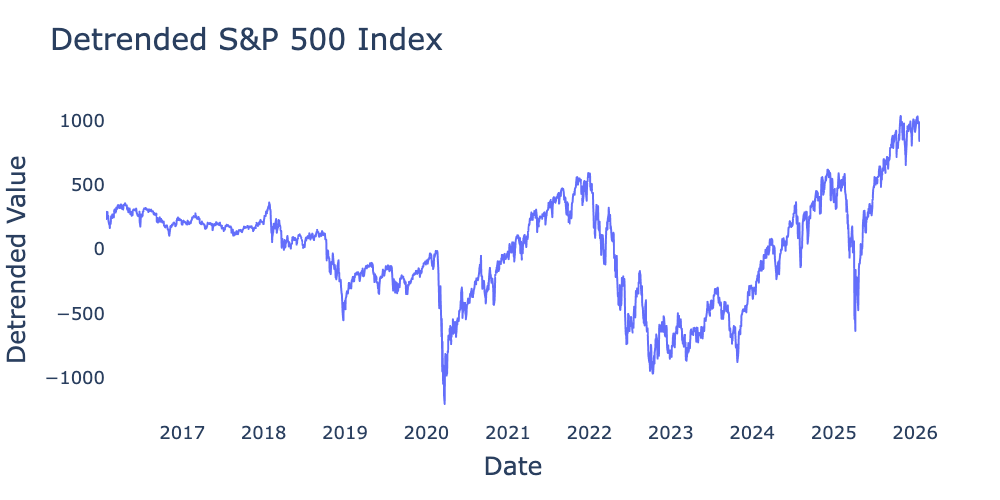
Detrended values of S&P 500 index for the 10-year period from January 2016 through January 2026 from Federal Reserve Bank of St. Louis detrended using \text{SP500}_{detrended} = \text{SP500} - 1645 - 1.66\,t. — Figure 1:Detrended values of S&P 500 index for the 10-year period from January 2016 through January 2026 from Federal Reserve Bank of St. Louis detrended using $\text{SP500}_{detrended} = \text{SP500} - 1645 - 1.66\,t$ .

What would happen if we instead take the first difference? pandas has a diff method accessed by df.diff(periods=1). Running the code

# Pandas uses periods=1 by default.
sp_500_diff = sp_500_df.diff().dropna()

we can use the differenced time series to create Figure 2

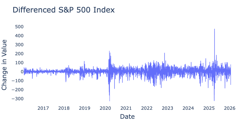
Figure 2:First difference of values of S&P 500 index for the 10-year period from January 2016 through January 2026 from Federal Reserve Bank of St. Louis.

Figure 2 appears more likely to be stationary than Figure 1, though I would caution against relying too heavily on pure visual inspection for either trends or overall stationarity. The mean of the differenced S&P 500 is 1.93, fairly close to the linear regression slope of 1.66. Figure 2 does appear to exhibit volatility clustering, which we will learn in subsequent chapters can be understood via the ARCH family of models. Nevertheless, it is reasonable to conclude that the S&P 500 roughly follows a random walk with drift of $\delta\approx1.9$ , making its first difference stationary white noise.

Autocorrelation of Random Walk¶

Before examining the autocorrelation, let’s work out what we expect the autocovariance of a random walk to look like. We’ve established that the autocovariance of a random walk is given by

\begin{aligned} \gamma(s,t) &= \text{Cov}\Big(\sum_{i=0}^s w_i, \sum_{j=0}^t w_j\Big)\\ &= \sum_{i=0}^{\text{min}(s,t)} \mathbb{V}(w_i)\\ &= \text{min}(s,t)\,\sigma_w^2. \end{aligned}

(21)

Translating to autocorrelation is a bit tricky as a random walk’s variance is non-constant. Standard statistical packages still use the sample approximation for $\gamma(h)$ and $\rho(h)$

\hat{\rho}(h) = \frac{\hat{\gamma}(h)}{\hat{\gamma}(0)}.

(22)

Even though Eq. (22) is only strictly valid for stationary time series, we can use it to approximate the autocorrelation for our case as well. Combining Eq.s (21) and (22) for a time series of length $t$ gives us

\begin{aligned} \hat{\rho}(h) &\approx \frac{\hat{\gamma}(s,t)}{\hat{\gamma}(t,t)}\\ &= \frac{\text{min}(s,t)\,\sigma_w^2}{t\,\sigma_w^2}\\ &= \frac{\text{min}(s,t)}{t}, \end{aligned}

(23)

which represents a linear decay as $h=t-s$ increases.

Do the autocorrelation functions agree with our assessment that the S&P 500 is a random walk? Let’s look at them:

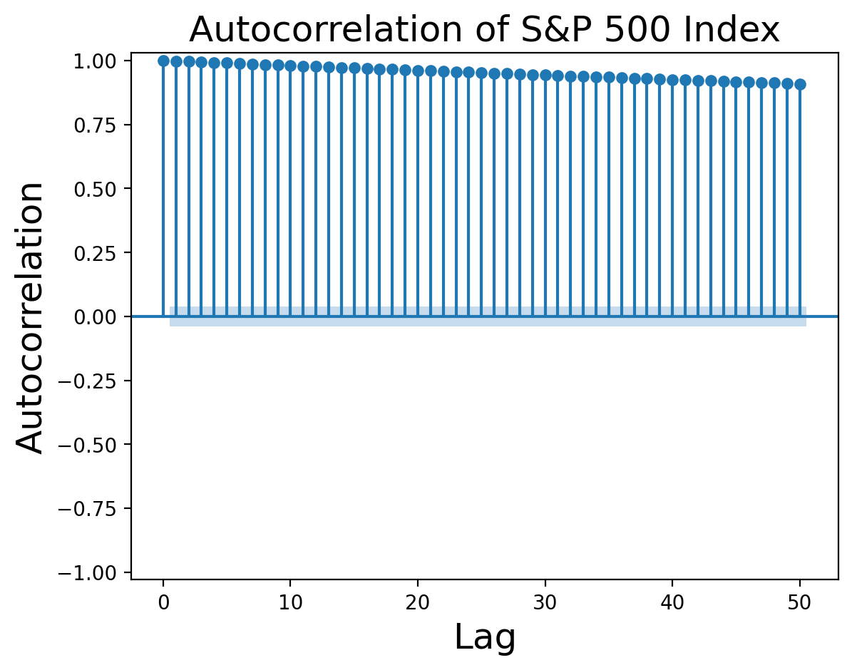
Figure 3:Autocorrelation function of S&P 500 returns from Federal Reserve Bank of St. Louis.

Figure 3 certainly looks like pure linear decay. What about the autocorrelation of the differenced series?

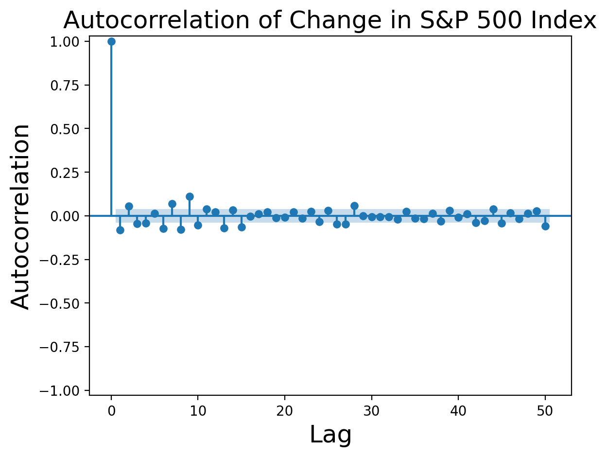
Figure 4:Autocorrelation function of first difference of S&P 500 returns from Federal Reserve Bank of St. Louis.

Multiple $h$ values before $h\approx15$ are significant beyond the level expected for pure white noise, indicating that our original process was probably not a pure random walk. Nevertheless, the autocorrelation values are small enough to say that a random walk is a reasonable first approximation to the S&P 500 returns.

Footnotes¶

We will discover other scenarios of difference stationary process where $\mu_t$ is not a simple random walk, but is a process possessing a unit root. We will defer discussion of these cases until after we have covered ARMA processes. For the time being, you can think of the concept of unit root as referring to random walks.
↩
Note that treating $\Delta t$ as 1 will cause the values to agree, but the units will not be the same. Eq. (10) includes units of $\text{time}^{-1}$ and Eq. (11) includes units of $\text{time}^{-2}$ .
↩
When we cover ARMA processes we will see that unnecessary differencing adds an additional moving average (MA) term and frequently results in non-invertible models.
↩