Definition of Trend
The first primary cause of non-stationarity we will discuss is the presence of a trend. At its most basic level, a trend is simply a long-term increase or decrease in values.
Recall from the first chapter that time series can exhibit highly convincing spurious trends. We will cover some statistical methods to determine if a trend is real in later chapters, but none of these are fool-proof. As a data scientist, you must always combine your prior domain knowledge to assist in determining if it is reasonable to assume the existence of a trend.
Trends and Detrending
S&P 500 Trend
The following plot of the S&P 500 values appears to exhibit a stable overall trend.
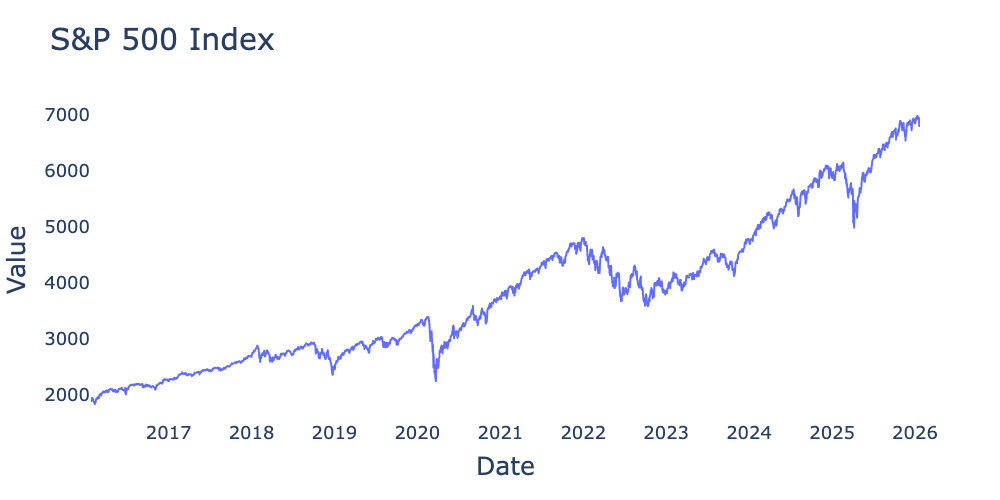
Figure 1:Raw values of S&P 500 index for the 10-year period from January 2016 through January 2026 from Federal Reserve Bank of St. Louis.
You can experiment with the values from Figure 1 by downloading the data using the following cell:
import pandas as pd
import matplotlib.pyplot as plt

df = pd.read_csv("https://fred.stlouisfed.org/graph/fredgraph.csv?bgcolor=%23ebf3fb&chart_type=line&drp=0&fo=open%20sans&graph_bgcolor=%23ffffff&height=450&mode=fred&recession_bars=on&txtcolor=%23444444&ts=12&tts=12&width=1320&nt=0&thu=0&trc=0&show_legend=yes&show_axis_titles=yes&show_tooltip=yes&id=SP500&scale=left&cosd=2016-01-25&coed=2026-01-23&line_color=%230073e6&link_values=false&line_style=solid&mark_type=none&mw=3&lw=3&ost=-99999&oet=99999&mma=0&fml=a&fq=Daily%2C%20Close&fam=avg&fgst=lin&fgsnd=2020-02-01&line_index=1&transformation=lin&vintage_date=2026-01-25&revision_date=2026-01-25&nd=2016-01-25",
                 index_col=0,
                 parse_dates=True,
                 )
# statsmodels is very particular regarding missing values, we will fill in missing values with the previous value.
df.ffill(inplace=True)
# examine a quick plot
plt.plot(df)
Trend Stationary Process
Given the apparent upward trend, it is reasonable to explore the possibility that the S&P 500 is trend stationary, i.e. the time series takes the form
where is the observed time series, is a trend, and is an underlying stationary time series. Eq. (1) suggests recovering via the process of detrending
What form should our estimate take? Let’s start with the most basic model, ordinary least squares (OLS)
where is the intercept and is the slope.
Detrending S&P 500
We will fit an OLS regression of the form in Eq. (3) using the following code:
import statsmodels.api as sm
import numpy as np

y = sp_500_df['SP500']
X = np.arange(len(sp_500_df))
# By default, statsmodels does not include an intercept term.
# We will add an intercept manually using add_constant.
X = sm.add_constant(X)

model = sm.OLS(y, X)
results = model.fit()

print(results.summary())
You should now see something like the following:
                            OLS Regression Results
==============================================================================
Dep. Variable:                  SP500   R-squared:                       0.907
Model:                            OLS   Adj. R-squared:                  0.907
Method:                 Least Squares   F-statistic:                 2.543e+04
Date:                Sun, 25 Jan 2026   Prob (F-statistic):               0.00
Time:                        18:33:02   Log-Likelihood:                -19337.
No. Observations:                2610   AIC:                         3.868e+04
Df Residuals:                    2608   BIC:                         3.869e+04
Df Model:                           1
Covariance Type:            nonrobust
==============================================================================
                 coef    std err          t      P>|t|      [0.025      0.975]
------------------------------------------------------------------------------
const       1644.6932     15.634    105.199      0.000    1614.037    1675.350
x1             1.6550      0.010    159.469      0.000       1.635       1.675
==============================================================================
Omnibus:                       10.728   Durbin-Watson:                   0.011
Prob(Omnibus):                  0.005   Jarque-Bera (JB):               10.076
Skew:                          -0.117   Prob(JB):                      0.00649
Kurtosis:                       2.806   Cond. No.                     3.01e+03
==============================================================================
Note that the is quite high, and both the intercept and slope are statistically significant.
Based on the results of our OLS, we will detrend the S&P 500 results using the formula
where consists of for observations. We can apply this formula using the code
detrend_component = results.params["const"] + results.params["x1"] * np.arange(len(sp_500_df))
sp_500_df_detrended = sp_500_df["SP500"] - pd.Series(detrend_component, index=sp_500_df.index)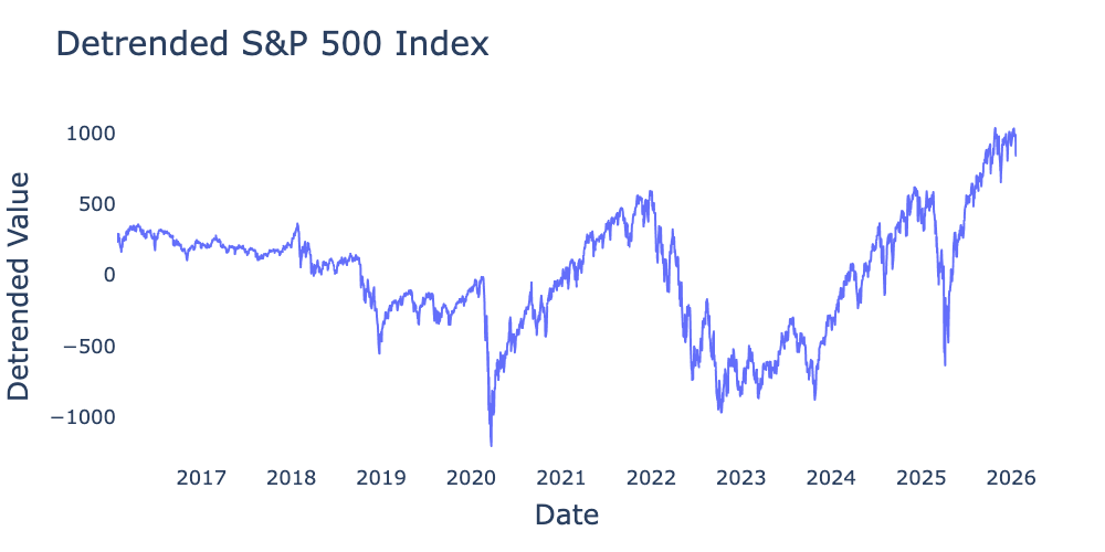
Figure 2:Detrended values of S&P 500 index for the 10-year period from January 2016 through January 2026 from Federal Reserve Bank of St. Louis detrended using .