Components of Time Series
Many time series contain trends, seasonal effects, and/or cycles. Time series decomposition, or simply decomposition, is defined as methods to isolate each component’s contribution to an overall time series. Since cycles lack a specific length it is difficult to draw a clear distinction between an upward trend followed by a downward trend and a cycle. Consequently, we will generally fold cycles into the trend for the purposes of decomposition.
Before diving into the details, let’s get a feeling for what a time series decomposition might look like.
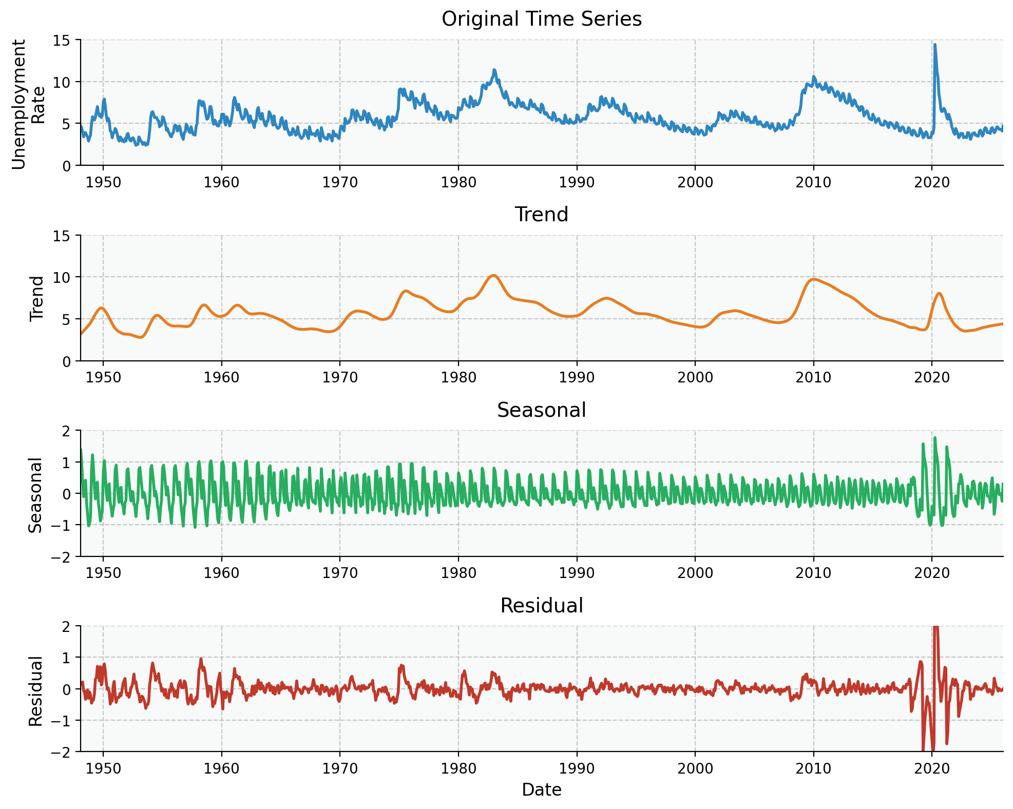
Figure 1:US employment rate from 1948 through 2025 from the Federal Reserve Bank of St. Louis with STL decomposition consisting of original series (top), trends and cycles (second from top), seasonal contribution (third from top), and residual variation not explained (bottom).
We’ll delve into the algorithms used to create figures like Figure 1 below and in subsequent chapters. For now, let’s take a moment to understand the components depicted in Figure 1.
: The trend component, consisting of both trends and cycles in the data.
: The seasonal component, consisting of regular periodicity at a specified seasonal length. Note that most decomposition methods only allow a single seasonality.
: The residual (sometimes also referred to as the remainder), consisting of any variation not accounted for by or . The residual can be thought of as roughly equivalent to noise , though I’d caution against taking this analogy too far. is only strictly equivalent to noise if and are a perfect model for the underlying process.
Additive and Multiplicative Models
Most commonly, we assume an additive decomposition in the form of
In some cases, we may also assume a multiplicative decomposition
which is more applicable, for example, in forecasting quarterly sales of a product experiencing compound growth in demand such as Mac sales in the previous chapter. Note that we can always recast Eq. (2) into the form of Eq. (1) by using a log transform
While other models are possible (see Hyndman (2004)), for example
such models are almost never used in practice if for no other reason than that the difficulty in interpreting the output can easily defeat the original purpose of time series decomposition.
Classical Decomposition Algorithm
Defining Seasonal Length
Before using the algorithm we must first define our seasonal period . Common values of include for weekly data, for monthly data, and for hourly data. Note that we cannot define multiple seasonal effects in a given decomposition.
Recall that a moving average with the length of a season (or any multiple thereof) will remove seasonal effects, allowing us to focus on longer term cycles and trends. For seasonal effects with odd numbers of time steps per season such as a for weekly seasonality, we employ a simple centered moving average of length . Thus, for data starting on a Sunday, the first Wednesday will be replaced with the average of the first Sunday-Saturday, the first Thursday will be replaced by the average of the the first Monday-Sunday, and so on. Note the we do lose the first and last observations for odd or—as we will see shortly—the first and last for even . This is not an issue for long time series in which the number of observations , but does pose a challenge for shorter time series.
Day Moving Average for Weeks
| Original Day of Week (Week Number) | Value in Smoothed Series |
|---|---|
| Sunday (1) | — |
| Monday (1) | — |
| Tuesday (1) | — |
| Wednesday (1) | |
| Thursday (1) | |
| Friday (1) | |
| Monday () | |
| Tuesday () | |
| Wednesday () | |
| Thursday () | — |
| Friday () | — |
| Saturday () | — |
For even values of such as quarterly data, it is impossible to center a moving average of length . As a compromise, we use a moving average. A moving average is a moving average of moving averages, for example, a moving average is defined as:
A moving average allows us to center each observation by using an odd length window, weighting the first and last observation by and the others by .
Quarterly Moving Average for Years
| Original Quarter (Year Number) | Value in Smoothed Series |
|---|---|
| First (1) | — |
| Second (1) | — |
| Third (1) | |
| Fourth (1) | |
| First () | |
| Second () | |
| Third () | — |
| Fourth () | — |
The smoothed series is used as our estimate of the series trend , denoted as to emphasize that it is an estimate to the true . From here on, classical decomposition subdivides into additive and multiplicative methods.
Additive Method
Having obtained our estimate of the trend , we are now ready to estimate the seasonality. We first detrend the series by subtracting
We then obtain our estimate of the seasonal component by taking the average of each detrended value of that season (e.g. the average detrended Thursday or average detrended May). The individual seasonal components are adjusted for an overall baseline of zero, i.e.
For example, our baseline temperature might be , with the summer being higher and the winter lower.
Having obtained our estimates and , the estimated residual is simply what’s left after subtracting the estimated trend and seasonality
Multiplicative Methods
In certain scenarios, in particular with time series exhibiting exponential growth, a multiplicative decomposition may be more appropriate. While we can always apply additive decomposition to the logarithm of the original series, classical decomposition is capable of directly estimating the multiplicative decomposition (Eq. (2)).
As with the additive case, we begin by obtaining our estimated trend via a moving average. We detrend the series via division
We obtain our estimated seasonal component by averaging each detrended season as before. For multiplicative decomposition the individual seasonal components are adjusted for a baseline of one, i.e.
For example the first quarter might have a seasonal component value of while the third quarter might have a component value of .
The residual is simply what remains after dividing out the estimated trend and seasonal effects
Plotting Decomposition Components
Above, we accessed the components of the classical decomposition and plotted them individually. statsmodels does have a nice feature to automatically plot the full decomposition invoked (using the variable names from above) as follows:
classic_decomp.plot()This should provide you with a plot like
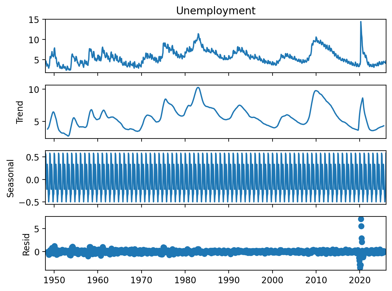
Figure 2:US employment rate from 1948 through 2025 from the Federal Reserve Bank of St. Louis with additive classical decomposition consisting of original series (top), trends and cycles (second from top), seasonal contribution (third from top), and residual variation not explained (bottom).
Assessing Decomposition Quality
A natural question to ask is how to assess the quality of a time series decomposition. Assuming that Eq. (1) or Eq. (2) is a reasonable model of the underlying data, a better decomposition can be expected to result in an estimated residual far smaller than the trend and seasonal components. While visual inspection of a plot such as Figure 2 or Figure 1 (paying careful attention to the scale of the y-axes!) is a valuable starting point, in certain scenarios we may wish to have a more quantitative metric.
Hyndman et al. (2026) recommend the following formula for estimating the strength of the trend
the logic being that for a time series with a strong trend component, the variance of the residual component alone should be much smaller than the variance of the combined trend and residual components. Thus, for data with a strong trend that has been well isolated by , will be close to 1. will be close to 0 for data with a minimal trend and/or a poorly isolated [1].
Computing from the unemployment data above using the formula
max(0, 1-(np.var(classic_decomp.resid)/np.var(classic_decomp.trend+classic_decomp.resid)))gives a value of 0.928, indicating a strong trend component that has been well isolated by .
The strength of the seasonal component is computed in the same manner as using the equation
Calculating using the code
max(0, 1-(np.var(classic_decomp.resid)/np.var(classic_decomp.seasonal +classic_decomp.resid)))gives a value of 0.379. While not terrible, compared to this value indicates either (1) a weaker seasonal component (unlikely based on visual examination of the original data), or that (2) our decomposition has not done as good a job isolating the seasonal component, resulting in having a weaker contribution to the estimated decomposition shown in Figure 2.
Drawbacks to Classical Decomposition
While not a terrible method, classical decomposition does have a number of drawbacks that make algorithms such as STL preferable. The major issues (highlighted in the derivations and exercises above) are as follows:
Use of a moving average removes the first and last ( even) or ( odd) observations from the trend (and consequently also the seasonal and residual components). For short time series this will result in sacrificing a fair amount of potential insight into the time series’ behavior.
Averaging each season across the data assumes there is exactly one seasonal value per season that is constant across the entire time series, rather than allowing the seasonal contribution itself to be a function of time.
Classical decomposition is not robust to brief but extreme fluctuations such as the COVID pandemic and its effect on unemployment rates.
For these reasons, most statistics texts recommend against using the classical method for anything beyond a baseline to compare to more advanced methods. In the coming sections we will build on our analysis of classical decomposition to understand STL decomposition and how it addresses the issues above.
The quantity could conceivably be greater than 1 if and have a strong negative covariance. Eq. (12) ensures that by use of the maximum of 0 or the computed value.
- Hyndman, R. J. (2004). The interaction between trend and seasonality. International Journal of Forecasting, 20(4), 561–563. https://doi.org/10.1016/j.ijforecast.2004.03.005
- Hyndman, R. J., Athanasopoulos, G., Garza, A., Challu, C., Mergenthaler, M., & Olivares, K. G. (2026). Forecasting: Principles and Practice, the Pythonic Way. OTexts.