6.2 Autoregressive Models

We begin our journey into ARMA models by discussing autoregressive, or AR models (the “AR” in ARMA). As the name implies, AR models can be thought of as the application of linear regression to time series by regressing a time series onto lagged versions of itself^[1].

Random Walk to AR(1)¶

Recall that a random walk is a model in which each time step’s value is determined by the previous time step’s value plus random noise, i.e.

x_t = x_{t-1} + w_t.

(1)

A random walk is not stationary due to its non-constant variance, making AR models not applicable. However, we could imagine a slightly different time series defined as

x_t = \phi x_{t-1} + w_t, \qquad |\phi|<1.

(2)

AR(1) Stationarity¶

Eq. (2) is a first order autoregressive process, denoted as AR(1). We will demonstrate that Eq. (2) describes a stationary process by iterating backwards and examining the properties of the resulting iterated series:

\begin{split} x_t &= \phi x_{t-1} + w_t\\ &=\phi (\phi x_{t-2}+ w_{t-1}) + w_t\\ &=\phi^2 x_{t-2} + \phi w_{t-1} + w_t\\ &=\phi^2(\phi x_{t-3} + w_{t-2}) + \phi w_{t-1} + w_t\\ &\ldots\\ &=\sum_{j=0}^{\infty} \phi^j w_{t-j} \end{split}

(3)

In coming sections, we will learn that Eq. (3) is the infinite moving average, or MA( $\infty$ ) representation of an AR process. For our purposes, we can think of it as a way to shed light on the behavior of an AR process.

AR(1) Mean¶

From the last line of Eq. (3) , we conclude that the mean of an AR(1) process is

\begin{split} \mathbb{E}[x_t] &= \mathbb{E}\Big[\sum_{j=0}^{\infty} \phi^j w_{t-j}\Big]\\ &=\sum_{j=0}^{\infty} \phi^j \mathbb{E}[w_{t-j}]\\ &=0. \end{split}

(4)

AR(1) Autocovariance¶

The autocovariance can be derived analogously. For any stationary AR(1) process with zero mean, $\gamma(h) =\text{Cov}(x_{t+h}, x_t)$ . Should the mean not be zero, replace $x_t$ with $x_t-\mu_x$ . We can then derive $\gamma(h)$ as

\begin{split} \gamma(h) &=\text{Cov}(x_{t+h}, x_t)\\ &=\mathbb{E}\Big[\Big(\sum_{j=0}^{\infty}\phi^j w_{t+h-j}\Big)\Big(\sum_{k=0}^{\infty} \phi^k w_{t-k}\Big)\Big]\\ &=\mathbb{E} [(w_{t+h} + \ldots + \phi^h w_t + \phi^{h+1} w_{t-1} + \ldots)(w_t + \phi w_{t-1} + \ldots)]. \end{split}

(5)

Noting that the covariance for the $w_t$ ’s is $\text{Cov}(w_i, w_j) = \delta_{ij}\sigma_w^2$ , we can line up all non-zero contributions stemming from cross-terms where $w_{t+h−j}$ in the left series matches $w_{t-k}$ in the right series. This will require $h−j=−k$ i.e. $j=h+k$ , giving us

\begin{split} \gamma(h) &= \sigma_w^2 \sum_{k=0}^{\infty} \phi^{h+k} \phi^k\\ &=\sigma_w^2 \phi^h \sum_{k=0}^{\infty} \phi^{2k}\\ &=\sigma_w^2 \frac{\phi^h}{1-\phi^2}, \end{split}

(6)

where we have cast the autocovariance as an infinite geometric series. Provided that $\sigma_w^2$ is finite, Eq. (6) will be finite for all values of $h$ . Finally, the last line of Eq. (6) depends solely on the separation $h$ , completing the proof that Eq. (2) represents a stationary process.

AR(1) Autocorrelation¶

Recall that the autocorrelation $\rho(h)$ for a stationary process is given by

\rho(h)\stackrel{\triangle}{=}\frac{\gamma(h)}{\gamma(0)}.

(7)

Plugging in the result from Eq. (6), we obtain:

\begin{split} \rho(h) &= \frac{\sigma_w^2 \frac{\phi^h}{1-\phi^2}}{\sigma_w^2 \frac{1}{1-\phi^2}}\\ &= \phi^h \end{split}

(8)

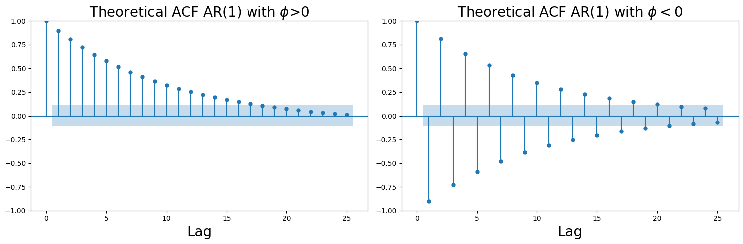
In the event that $\phi<0$ , $\rho(h)$ will also die off in a sinusoidal fashion, alternating between positive and negative values due to serial negative correlation. These two possibilities are demonstrated in Figure 1.

Theoretical autocorrelation for stationary AR(1) processes with \phi>0 and \phi<0. — Figure 1:Theoretical autocorrelation for stationary AR(1) processes with $\phi>0$ and $\phi<0$ .

Problem

We stated above that we cannot fit a non-stationary AR model, but we haven’t explained what the problem is. A full exploration of the problem with non-stationary models requires a deeper dive into the mathematical underpinnings of ARMA models; however, we can begin to see some of the problems by creating a few simulated time series in this exercise inspired by Granger & Newbold (1974). Run the following code to explore spurious correlations in random walks. Note that #%% denotes a new code cell.

import numpy as np
import plotly.express as px
#%%
np.random.seed(4400) # set seed for reproducibility
SIZE = 1000
#%%
# Create random walks by summing random noise.
rw_1 = np.cumsum(a=np.random.normal(loc=0, scale=1, size=SIZE))
rw_2 = np.cumsum(a=np.random.normal(loc=0, scale=1, size=SIZE))
print("Correlation between random walks: ", np.corrcoef(rw_1, rw_2)[1,0])
#%%
# examine quick plot
px.line(x=np.arange(SIZE), y=[rw_1, rw_2])
#%%
# In this cell we will create two AR(1) processes that are close to random walks in terms of phi values.
PHI = 0.95
ar1_1 = np.empty(SIZE)
ar1_1[0] = 0
for idx in range(1, SIZE):
    ar1_1[idx] = PHI*ar1_1[idx-1] + np.random.normal(loc=0, scale=1)
ar1_2 = np.empty(SIZE)
ar1_2[0] = 0
for idx in range(1, SIZE):
    ar1_2[idx] = PHI*ar1_2[idx-1] + np.random.normal(loc=0, scale=1)
print("Correlation between AR(1) processes: ", np.corrcoef(ar1_1, ar1_2)[1,0])
#%%
px.line(x=np.arange(SIZE), y=[ar1_1, ar1_2])

What happens if you run the code multiple times with different seeds? How frequently do you observe a spurious high correlation between the random walks? What about between the AR(1) processes?

AR(1) with Nonzero Mean¶

Up to this point, we’ve assumed that our AR(1) model has a mean of 0 (or that we subtracted the mean prior to our analysis), in which case $\phi$ exerts a sort of gravitational pull to bring values back to 0 by damping out previous noise. We can extend this to an AR(1) process with a nonzero mean $\mu$ by subtracting the mean from each observation in the AR model itself

\begin{split} x_t-\mu &= \phi(x_{t-1}-\mu) + w_t\\ x_t &= \phi x_{t-1} -\phi \mu + \mu + w_t\\ &= \phi x_{t-1} + (1-\phi)\mu + w_t\\ &= \alpha + \phi x_{t-1} + w_t, \end{split}

(9)

where $\alpha \stackrel{\triangle}=\mu(1-\phi)$ functions the same way that an intercept term would in standard linear regression.

AR( $p$ ) Models¶

It’s straightforward to generalize AR models to higher order AR( $p$ ) models with $p\geq1$ by regressing the time series onto versions of itself of increasing lag. A general AR( $p$ ) model is given as

x_t = \phi_1 x_{t-1} + \phi_2 x_{t-2} + \ldots + \phi_p x_{t-p} + w_t, \qquad \phi_p \neq 0.

(10)

A series with a nonzero mean is handled as

\begin{split} x_t-\mu &= \phi_1 (x_{t-1}-\mu) + \phi_2 (x_{t-2}-\mu) + \ldots + \phi_p (x_{t-p}-\mu) + w_t\\ x_t &= \mu(1-\phi_1-\phi_2-\ldots-\phi_p) + \phi_1 x_{t-1} + \phi_2 x_{t-2} + \ldots + \phi_p x_{t-p} + w_t\\ &= \alpha + \phi_1 x_{t-1} + \phi_2 x_{t-2} + \ldots + \phi_p x_{t-p} + w_t, \end{split}

(11)

where as before the intercept is given as $\alpha \stackrel{\triangle}=\mu(1-\phi_1-\phi_2-\ldots-\phi_p)$ .

Deriving the theoretical autocovariance and autocorrelation functions of an AR( $p$ ) process is somewhat more involved than for an AR(1) model. We will defer the derivation until after we have covered representing AR models as infinite series of noise terms in section 4.

AR Models in Backshift Notation¶

Autoregressive Operator¶

Recall from Eq. (14) in section 4.3 that the backshift operator $\mathbb{B}$ increments a time series back by one time step. Using this definition, we may express Eq. (2) as

\begin{split} &x_t = \phi\,\mathbb{B}\,x_{t} + w_t\\ &x_t - \phi\,\mathbb{B}\,x_{t} = w_t\\ &(1 - \phi\,\mathbb{B})\,x_{t} = w_t.\\ \end{split}

(12)

We can expand this definition to represent AR( $p$ ) models using backshift notation as

(1-\phi_1 \mathbb{B} - \phi_2 \mathbb{B}^2 -\ldots-\phi_p \mathbb{B}^p)x_t = w_t,

(13)

or in more compact form

\phi(\mathbb{B})x_t = w_t,

(14)

where $\phi(\mathbb{B})$ is the autoregressive operator defined as:

\phi(\mathbb{B}) \stackrel{\triangle}{=} 1-\phi_1 \mathbb{B} -\phi_2 \mathbb{B}^2 - \ldots - \phi_p \mathbb{B}^p.

(15)

For stationary AR models ( $|\phi|<1$ for AR(1)), we can define an inverse autoregressive operator $\phi^{-1}(\mathbb{B})$

\phi^{-1}(\mathbb{B})\phi(\mathbb{B})x_t = \phi^{-1}(\mathbb{B})w_t

(16)

x_t = \phi^{-1}(\mathbb{B})w_t.

(17)

For an AR(1) model, given that $\phi^{-1}(\mathbb{B}) = \frac{1}{1-\phi \mathbb{B}}$ and $|\phi|<1$ , we can represent $\phi^{-1}(\mathbb{B})$ as an infinite geometric series

\phi^{-1}(\mathbb{B}) = 1 + \phi \mathbb{B} + \phi^2 \mathbb{B}^2 + \phi^3 \mathbb{B}^3 + \ldots

(18)

Causal AR Models¶

What is the purpose of representing AR processes in the form of Eq. (13) or (14)? To answer this, begin by noting that Eq. (18) implies that $x_t = w_t + \phi w_{t-1} + \phi^2 w_{t-2}+\ldots$ , as derived in Eq. (3). This is an example of a causal model, in which a series can be treated as being generated by an infinite series of noise terms. Random walks, on the other hand, are non-causal as they will increase without bound as we include more and more time steps. Series with $|\phi|>1$ are referred to as explosive as past noise becomes arbitrarily magnified as $\phi$ is raised to increasing powers—exactly what happens in a physical explosion (at least until the fuel is exhausted).

Non-causal processes such as unit root and explosive processes are not stationary, making many of the tools used in time series analysis unsuitable. We can easily determine if an AR(1) process is causal by examining $\phi$ , how might we do the same for higher order AR( $p$ ) models? Imagine if we could factor an AR model such that

(1-\phi_1 \mathbb{B} - \phi_2 \mathbb{B}^2 -\ldots-\phi_p \mathbb{B}^p)x_t=(1-\varphi_1^{\prime} \mathbb{B})(1-\varphi_2^{\prime} \mathbb{B})\ldots(1-\varphi_p^{\prime} \mathbb{B})x_t.

(19)

Given such a factoring, we could quickly determine if our AR( $p$ ) model was causal—and hence stationary—simply by confirming that all $\varphi^{\prime}$ 's have an absolute value less than 1. While there is no guarantee this will be possible for real $\varphi^{\prime}$ 's, the fundamental theorem of algebra does ensure this is possible for complex values^[2].

Let’s explore this with an concrete example. Consider the second order autoregressive, or AR(2), model defined as

x_t = 1.25x_{t-1} - 0.375 x_{t-2} + w_t.

(20)

Looking at Eq. (20), it’s not immediately obvious if its $\varphi^{\prime}$ 's are greater than one. Let’s recast it using the autoregressive operator $\phi(\mathbb{B})$

\begin{split} x_t = 1.25\,x_{t-1} - 0.375\, x_{t-2} + w_t\\ x_t - 1.25\,x_{t-1} + 0.375\, x_{t-2} = w_t\\ (1-1.25\,\mathbb{B} + 0.375\,\mathbb{B}^2)x_t = w_t. \end{split}

(21)

Evidently, $\phi(\mathbb{B})=1-1.25\,\mathbb{B} + 0.375\,\mathbb{B}^2=1-\frac{5}{4}\,\mathbb{B} + \frac{3}{8}\,\mathbb{B}^2$ . Now comes the crucial step, we replace the backshift operator with a variable, call it $z$ , and solve for the zeros of the polynomial $\phi(z)$ .

\begin{split} 1-\frac{5}{4}\,z + \frac{3}{8}\,z^2 &= 0\\ (1-\frac{1}{2}\,z)(1-\frac{3}{4}\,z) &= 0\\ z = 2 \quad \text{or} \quad z=\frac{4}{3}. \end{split}

(22)

Eq. (20) is stationary because the $\varphi^{\prime}$ 's of $\frac{1}{2}$ and $\frac{3}{4}$ have absolute values less than one (lie inside the unit circle^[3]). Equivalently, the roots of $\phi(z)$ (and consequently of $\phi(\mathbb{B})$ ) of 2 and $\frac{4}{3}$ have absolute values greater than one (lie outside the unit circle).

Sign of $\phi$ and Complex Roots¶

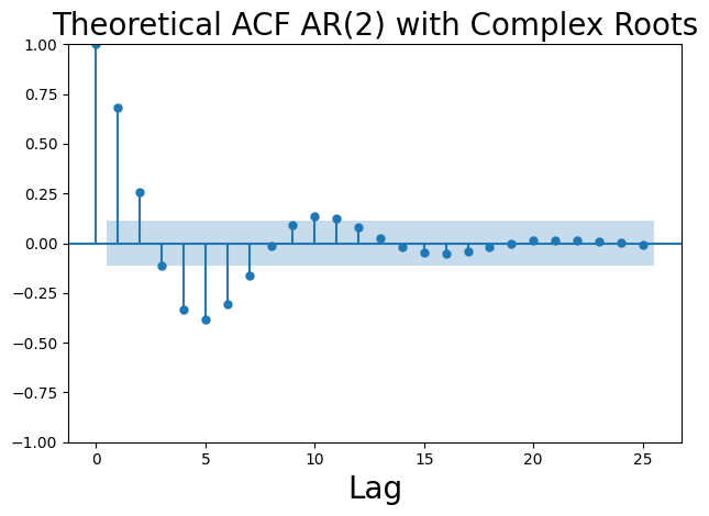
As seen above, the signal characteristic of stationary AR models is the presence of exponentially decaying autocovariance (and consequently autocorrelation) functions. For an AR( $p$ ) process with $p\geq2$ , the decay may also exhibit sinusoidal oscillations, potentially with a period greater than $p$ .

Figure 2:Theoretical autocorrelation for stationary AR(2) processes with complex roots.

If the above fails to render correctly in your browser you can also open the demo as a new browser window using the Open Demo in a New Tab ↗ button at the top of the frame. Note that you may need to enable popups for this to work.

By the quadratic formula, an AR(2) process with associated polynomial $\phi(z)=1-\phi_1 z - \phi_2 z^2$ will be stationary only if

\Bigg|\frac{\phi_1\pm\sqrt{\phi_1^2+4\phi_2}}{-2\phi_2}\Bigg| > 1

(23)

Eq. (23) can be broken into three distinct requirements:

$\phi_1 + \phi_2 < 1$
$\phi_2 - \phi_1 < 1$
$\phi_2 > -1$

Some sources state the third requirement as $|\phi_2|<1$ , though this is not strictly necessary as combining the first two requirements above already enforces $\phi_2<1$ .

From Eq. (23) we see that the roots of an AR(2) model will be complex if $\phi_1^2+4\phi_2<0$ , i.e. if $\phi_2<-\frac{\phi_1^2}{4}$ . In Sec. 4 of this chapter we will see that AR processes with complex roots have a special property of exhibiting a “pseudo-seasonality.” These conditions are depicted in the Figure 3.

Values of \phi_1 and \phi_2 for AR(2) process demonstrating the boundary conditions for stationarity and real/complex roots. — Figure 3:Values of $\phi_1$ and $\phi_2$ for AR(2) process demonstrating the boundary conditions for stationarity and real/complex roots.

Higher Order Causal Models¶

We could expand the process above for finding unit roots in AR(2) models to higher order AR( $p$ ) models, but in practice there’s no need to do this by hand. statsmodels.tsa.arima_process.ArmaProcess provides theoretical properties of AR (and more broadly ARMA) models for us. The following code demonstrates using this module both to determine stationarity writ large and to extract the roots of an AR model. Note that the sign convention follows $\phi(\mathbb{B})$ from Eq. (21), not Eq. (20).

from statsmodels.tsa.arima_process import ArmaProcess
ar2 = ArmaProcess(ar=[1, -1.25, 0.375], # use phi values defined via phi(B)
                  ma = None, # pure AR process, no MA component
                 )
print(f"AR(2) model is stationary: {ar2.isstationary}")
print(f"Roots of AR(2) model: {ar2.arroots}")

Where do AR Processes Arise?¶

In economics are related disciplines, AR models are often referred to as “long-memory” models. This makes sense, as exponentially decaying autocorrelation means that a noise term, or “shock,” will take many steps to be “forgotten” (i.e. fade to statistical insignificance). Such a model is appropriate for a wide range of scenarios, ranging from climate science to economic inflation and stock market returns. In the following problem, we will explore using AR processes to get a baseline approximation to solar activity.

Problem

In this problem we will explore fitting AR( $p$ ) models to the sunspots dataset the comes with statsmodels and using both AIC and BIC to rank solutions.

import numpy as np
import pandas as pd
import plotly.express as px
from statsmodels.datasets import sunspots
from statsmodels.tsa.arima.model import ARIMA
from statsmodels.tsa.arima_process import ArmaProcess
#%%
print(sunspots.NOTE)
#%%
sunspots_df = sunspots.load_pandas().data
sunspots_df["YEAR"] = pd.to_datetime(sunspots_df["YEAR"], format='%Y', )
sunspots_df.set_index("YEAR", inplace=True, drop=True)
sunspots_df = sunspots_df.asfreq('YS') # Explicitly set the frequency to 'Year Start'
sunspots_df.head()
#%%
# examine quick plot
px.line(sunspots_df)
#%%
# create and save AR(p) models for p=1,2,3,4
ar_model_dict = {}
for p in range(1,5):
  print(f"AR Model for p={p}")
  ar_model_dict[p] = ARIMA(sunspots_df, order=(p,0,0)).fit()
  print("AIC: ", ar_model_dict[p].aic)
  print("BIC: ", ar_model_dict[p].bic)
  print("\n")

You should see that the AR(1) performs notably worse, wheres the AR(2), AR(3), and AR(4) models are roughly tied. AIC slightly favors the AR(3), whereas (consistent with its tendency to choose more parsimonious models) BIC very slightly favors the AR(2), though in both cases the difference between models for $p>1$ is small enough that I wouldn’t read too much into it. Let’s look at a summary and the theoretical properties of the AR(2) model. Don’t worry if you’re not yet familiar with some of the terms in the summary, we’ll get to the relevant ones in subsequent sections.

# print model summary
ar_model_dict[2].summary()
#%%
# create a theoretical ARMA model to explore its properties
phi_1 = ar_model_dict[2].params['ar.L1']
phi_2 = ar_model_dict[2].params['ar.L2']
ar2 = ArmaProcess(ar=[1, -phi_1, -phi_2], # note change of sign of phi values
                  ma = None, # pure AR process, no MA component
                 )
print(f"AR(2) model is stationary: {ar2.isstationary}")
print(f"Roots of AR(2) model: {ar2.arroots}")
# get pseudo-periodicity
print(f"Pseudo-period: {round(2*np.pi/np.abs(np.angle(ar2.arroots[0])), 2)} years")

Is the pseudo-period consistent with the plot from above?

Next, let’s compare the sample autocovariance to the theoretical autocovariance of our proposed AR(2) model.

sample_acf = plot_acf(sunspots_df, title="Sample ACF")
sample_acf.show()

theoretical_acf_plot = plot_acf(ar2.acf(), adjusted=False, title='Theoretical ACF')
theoretical_acf_plot.show()

Do the two plots appear to agree?

Finally, let’s explore using statsmodels to generate one-step-ahead in-sample predictions and recursively forecast the next 22 years out-of-sample. Don’t worry if you don’t get everything in this cell, we’ll revisit predicting and forecasting in subsequent sections.

# In this cell we will begin exploring using AR models for prediction.
# We will first fit perform one-step-ahead prediction throughout the observation window, followed by recursive prediction for the following 22 years.
pred = ar_model_dict[2].get_prediction(dynamic=False) # one-step-ahead prediction for in-sample data
forecast = ar_model_dict[2].get_forecast(22) # forecast for out-of-sample data
pred_df = pd.DataFrame(index=pred.predicted_mean.index.append(forecast.predicted_mean.index),
                       columns=["Observed", "One-Step-Ahead-Forecast"],
                       )
pred_df["Observed"] = sunspots_df
pred_df["One-Step-Ahead-Forecast"] = pd.concat([pred.predicted_mean, forecast.predicted_mean])
px.line(pred_df)

Does the in-sample prediction seem reasonable? What about the out-of-sample forecast?

Footnotes¶

Yule’s original 1927 paper (Yule (1927)) introducing autoregressive models motivated the concept by drawing an analogy to a randomly perturbed oscillatory system—in effect discretizing the differential equations governing damped harmonic oscillators (though Yule himself did not directly use differential equation terminology). Modern students coming from a data science or statistics background are generally more comfortable interpreting AR models as form of linear regression in which the features are lagged versions of the time series itself.
↩
The fundamental theorem of algebra states that any polynomial of degree $p$ has exactly $p$ roots (provided we allow for complex roots). The theorem allows for a single root to appear multiple times such as in the case of $1+2x+x^2=(1+x)^2$ , which has the root $x=-1$ with multiplicity 2.
↩
The unit circle is simply the set of all complex numbers such that $|a+bi|=1$ , or equivalently all complex numbers of the form $e^{i\theta},\, \theta\in[0,2\pi)$ .
↩
The actual requirement is derived by using the reciprocal definition of the roots $z$ from the definition we used. Our definition using $\varphi^{\prime}$ expresses the same idea from a different angle.
↩

References¶

Granger, C. W. J., & Newbold, P. (1974). Spurious regressions in econometrics. Journal of Econometrics, 2(2), 111–120. https://doi.org/10.1016/0304-4076(74)90034-7
Shumway, R. H., & Stoffer, D. S. (2025). Time Series Analysis and Its Applications. In Springer Texts in Statistics. Springer Nature Switzerland. 10.1007/978-3-031-70584-7
Yule, G. U. (1927). VII. On a method of investigating periodicities disturbed series, with special reference to Wolfer’s sunspot numbers. Philosophical Transactions of the Royal Society of London. Series A, Containing Papers of a Mathematical or Physical Character, 226(636–646), 267–298.